We present here the augmented Lagrangian method for solving systems arising from mixed finite element discretization of elliptic boundary value problem:
|
| (1.1) |
The aim is to show that implementing an efficient iterative method for the resulting indefinite linear system reduces to designing an efficient method for the solution of an auxiliary nearly singular H(div) problem.
The model problem (1.1) can be casted into the following mixed problem by
introducing the variable u := ∇p: Find (u,p)  H(div) × L2(Ω) such that
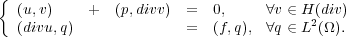 | (1.2) |
Given a conforming triangulation  h, the mixed finite element method is to solve the
model problem (1.2) in the finite element spaces: V h(div) ⊂ H(div) and V h(0) ⊂ L2(Ω).
That is,to find (uh,ph) V h(div) × V h(0) such that
h, the mixed finite element method is to solve the
model problem (1.2) in the finite element spaces: V h(div) ⊂ H(div) and V h(0) ⊂ L2(Ω).
That is,to find (uh,ph) V h(div) × V h(0) such that
 | (1.3) |
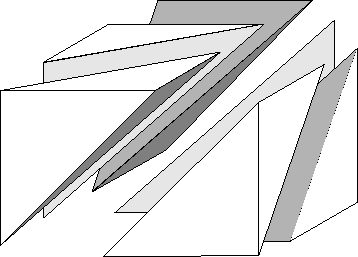
Here we restrict ourselves to the lowest order Raviart-Thomas spaces for V h(div).
The mixed finite element method (1.3) results in the following linear system:
![[A B*][u] [0]
B 0 p = f .](mixed3x.png) | (1.4) |
It is not difficult to see that A is the mass matrix of the Raviart-Thomas element and B is the matrix representations of div*.
The augmented Lagrangian method solves the following equivalent problem to (1.4) by the Uzawa method:
![[ ][ ] [ ]
A + ϵ-1B*B B * u ϵ-1B*f
B 0 p = f .](mixed4x.png) | (2.1) |
The iteration reads: Given (u(k),p(k)), the new iterate (u(k+1),p(k+1)) is obtained by solving the following systems:
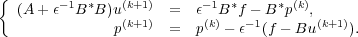 | (2.2) |
This algorithm has the following convergence.
Theorem 2.1. Let (u(0),p(0)) be a given initial guess and for k ≥ 1, let (u(k),p(k)) be the iterates obtained via the augmented Lagrangian method. Then the following estimates hold:
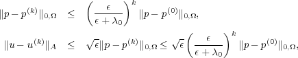
According to this theorem, the iteration procedure (2.2) converges very fast to the solution of (1.3) for small ϵ. However, one needs to solve a nearly singular H(div) system
 | (2.3) |
Thus, an efficient and robust H(div) solver will result in an optimal iterative method for the saddle point problem (1.3). For the nearly singular H(div) system (2.3), we used auxiliary AMG solver.
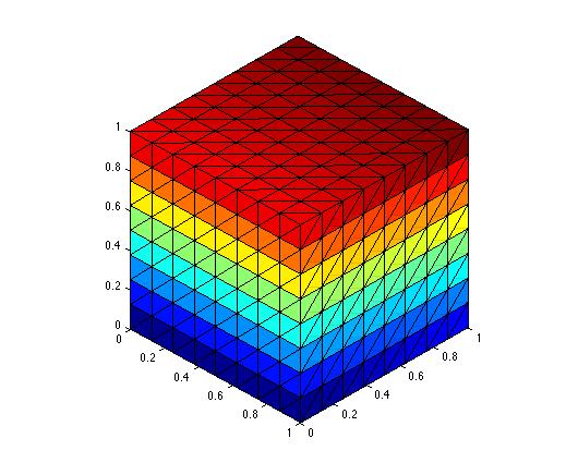
Here, we solve equation (1.1) in a unit cube [0,1]3 with structured tetrahedra mesh. The right hand side f = 1. Each cube is partitioned into 6 tetrahedrons.
|
|