Chapter 3 Data Objects, Packages, and Datasets

"In God we trust. All others [must] have data."

- Edwin R. Fisher, cancer pathologist

3.1 Data Storage Objects

There are five primary types of data storage objects in R. These are: (atomic) vectors, matrices, arrays, dataframes, and lists¹.

3.1.1 Atomic Vectors

Atomic vectors contain data with order and length, but no dimension. This is clearly different from the linear algebra conception of a vector. In linear algebra, a row vector with $n$ elements has dimension $1 \times n$ (1 row and $n$ columns), whereas a column vector has dimension $n \times 1$.

We can create atomic vectors with the function c.

x <- c(1, 2, 3)
is.vector(x)

[1] TRUE

length(x)

[1] 3

dim(x)

NULL

We can add a names attribute to vector elements. For example,

x <- c(a = 1, b = 2, c = 3)
x

a b c 
1 2 3

attributes(x)

$names
[1] "a" "b" "c"

attr(x, "names") # or  names(x)

[1] "a" "b" "c"

The function as.matrix(x) can be used to coerce x to have a matrix structure with dimension $3 \times 1$ (3 rows and 1 column). Thus, in R a matrix has dimension, but a vector does not.

dim(as.matrix(x))

[1] 3 1

Recall (Ch. 2) that an object’s base type defines the (R internal) type or storage mode of any object. Recall further that the 25 base types include "integer", "double", "complex", and "character" (Table ??). Elements of vectors must have a single data storage mode. Thus, a vector cannot contain both numeric and categorical (i.e., character) data.

Importantly, when an element-wise operation is applied to two unequal length vectors, R will generate a warning and automatically recycle elements of the shorter vector. For instance:

c(1, 2, 3) + c(1, 0, 4, 5, 13)

Warning in c(1, 2, 3) + c(1, 0, 4, 5, 13): longer object length is not a
multiple of shorter object length

[1]  2  2  7  6 15

In this case, the result of the addition of the two vectors is: $1 + 1, 2 + 0, 3 + 4, 1 + 5$, and $2 + 13$. Thus, the first two elements in the first object are recycled in the vector-wise addition.

3.1.2 Matrices

Matrices are two-dimensional (row and column) data structures whose elements all have the same data storage mode (typically "double").
The function matrix() can be used to create matrices:

A <- matrix(ncol = 2, nrow = 2, data = c(1, 2, 3, 2))
A

     [,1] [,2]
[1,]    1    3
[2,]    2    2

Matrix algebra operations can be applied directly to R matrices (Table 3.1). More complex matrix analyses are also possible, including eigenanalysis (function eigen()), and single value, QR, and Cholesky decompositions (the functions eigen(), svd(), chol(), respectively).

Table 3.1: Simple matrix algebra operations in R. In all operations $\boldsymbol{A}$ (and correspondingly, `A`) is a matrix
Operator	Operation	To.find.	We.type.
`t()`	Matrix transpose	$\boldsymbol{A}^T$	`t(A)`
`%*%`	Matrix multiply	$\boldsymbol{A} \cdot \boldsymbol{A}$	`A%*%A`
`det()`	Determinant	$Det(\boldsymbol{A})$	`det(A)`
`solve()`	Matrix inverse	$\boldsymbol{A}^{-1}$	`solve(A)`

t(A)

     [,1] [,2]
[1,]    1    2
[2,]    3    2

A %*% A

     [,1] [,2]
[1,]    7    9
[2,]    6   10

det(A)

[1] -4

solve(A)

     [,1]  [,2]
[1,] -0.5  0.75
[2,]  0.5 -0.25

We can use the function cbind() to combine vectors into matrix columns,

a <- c(1, 2, 3); b <- c(2, 3, 4)
cbind(a, b)

     a b
[1,] 1 2
[2,] 2 3
[3,] 3 4

and use the function rbind() to combine vectors into matrix rows.

rbind(a,b)

  [,1] [,2] [,3]
a    1    2    3
b    2    3    4

3.1.3 Arrays

Arrays are one, two dimensional (matrix), or three or more dimensional data structures whose elements contain a single type of data. Thus, while all matrices are arrays, not all arrays are matrices.

class(A)

[1] "matrix" "array"

As with matrices, elements in arrays can have only one data storage mode.

typeof(A) # base type (data storage mode)

[1] "double"

The function array() can be used to create arrays. The first argument in array() defines the data. The second argument is a vector that defines both the number of dimensions (this will be the length of the vector), and the number of levels in each dimension (numbers in dimension elements). For instance, here is a $2 \times 2 \times 2$ array.

some.data <- c(1, 2, 3, 4, 5, 6, 7, 8)
B <- array(some.data, c(2, 2, 2))
B

, , 1

     [,1] [,2]
[1,]    1    3
[2,]    2    4

, , 2

     [,1] [,2]
[1,]    5    7
[2,]    6    8

class(B)

[1] "array"

3.1.4 Dataframes

Dataframes are two-dimensional structures whose columns can be have different data storage modes (e.g. quantitative or categorical). The function data.frame() can be used to create dataframes.

df <- data.frame(numeric = c(1, 2, 3), non.numeric = c("a", "b", "c"))
df

  numeric non.numeric
1       1           a
2       2           b
3       3           c

class(df)

[1] "data.frame"

Because of the possibility of different data storage modes for distinct columns, the data storage mode of a dataframe is "list". Specifically, a dataframe is a list, whose storage elements are columns.

typeof(df)

[1] "list"

A names attribute will exist for each dataframe column².

names(df)

[1] "numeric"     "non.numeric"

The $ operator allows access to dataframe columns.

df$non.numeric

[1] "a" "b" "c"

The function attach() allows R to recognize column names of a dataframe as global variables.

attach(df)
# non.numeric  --allows retrieval of non.numeric directly

The function detach() is the programming inverse of attach().

detach(df)
# non.numeric  --produces error

The functions rm() and remove() will entirely remove any R-object, including a vector, matrix, or dataframe from a session. To remove all objects from the workspace one can use rm(list=ls()) or (in RStudio) the “broom” button in the The environments and history panel³.

A safer alternative to attach() is the function with(). Using with() eliminates concerns about multiple variables with the same name becoming mixed up in functions. This is because the variable names for a dataframe specified in with() will not be permanently attached in an R-session.

with(df, non.numeric)

[1] "a" "b" "c"

3.1.5 Lists

Lists are often used to contain miscellaneous associated objects. Like dataframes, lists need not use a single data storage mode. Unlike dataframes, however, lists can include objects that are not two-dimensional or with different data classes including character strings (i.e., units of character objects), multiple matrices and dataframes with varying dimensionality, and even other lists. The function list() can be used to create lists.

ldata1 <- list(a = c(1, 2, 3), b = "this.is.a.list")
ldata1

$a
[1] 1 2 3

$b
[1] "this.is.a.list"

class(ldata1)

[1] "list"

typeof(ldata1)

[1] "list"

Objects in lists can be called using the $ operator. Here is the character string b from ldata.

ldata1$b

[1] "this.is.a.list"

We note that to create an R-object containing character strings, we need to place quotation marks around entries.

x <- c("low", "med", "high")
x

[1] "low"  "med"  "high"

The function str attempts to display the internal structure of an R object. It is extremely useful for succinctly displaying the contents of complex objects like lists.

str(ldata1)

List of 2
 $ a: num [1:3] 1 2 3
 $ b: chr "this.is.a.list"

We are told that ldata1 is a list containing two objects: a sequence of numbers from 1 to 3, and a character string.

The function do.call() is useful for large scale manipulations of data storage objects. For example, what if you had a list containing multiple dataframes with the same column names that you wanted to bind together?

ldata2 <- list(df1 = data.frame(lo.temp = c(-1,3,5), high.temp = c(78, 67, 90)),
              df2 = data.frame(lo.temp = c(-4,3,7), high.temp = c(75, 87, 80)),
              df3 = data.frame(lo.temp = c(-0,2), high.temp = c(70, 80)))

You could do something like:

do.call("rbind",ldata2)

      lo.temp high.temp
df1.1      -1        78
df1.2       3        67
df1.3       5        90
df2.1      -4        75
df2.2       3        87
df2.3       7        80
df3.1       0        70
df3.2       2        80

Or what if I wanted to replicate the df3 dataframe from ldata above, by binding it onto the bottom of itself three times? I could do something like:

do.call("rbind", replicate(3, ldata2$df3, simplify = FALSE))

  lo.temp high.temp
1       0        70
2       2        80
3       0        70
4       2        80
5       0        70
6       2        80

Note the use of the function replicate().

3.2 Boolean Operations

Computer operations that dichotomously classify true and false statements are called logical or Boolean. In R, a Boolean operation will always return one of the values TRUE or FALSE. R logical operators are listed in Table 3.2.

Table 3.2: Logical (Boolean) operators in R; `x`, `y`, and `z` in columns three and four are R objects.
Operator	Operation	To ask:	We type:
`>`	$>$	Is `x` greater than `y`?	`x > y`
`>=`	$\geq$	Is `x` greater than or equal to `y`?	`x >= y`
`<`	$<$	Is `x` less than `y`?	`x < y`
`<=`	$\leq$	Is `x` less than or equal to `y`	`x <= y`
`==`	$=$	Is `x` equal to `y`?	`x == y`
`!=`	$\neq$	Is `x` not equal to `y`?	`x != y`
`&`	and	Do `x` and `y` equal `z`?	`x & y == z`
`&&`	and (control flow)	Do `x` and `y` equal `z`?	`x && y == z`
\|	or	Do `x` or `y` equal `z`?	`x` \| `y == z`
\|\|	or (control flow)	Do `x` or `y` equal `z`?	`x` \|\| `y == z`

Note that there are two ways to specify “and” (& and &&), and two ways to specify “or” (| and ||). The longer forms of “and” and “or” evaluate queries from left to right, stopping when a result is determined. Thus, this form is more appropriate for programming control-flow operations.

Example 3.1
For demonstration purposes, here is a simple dataframe:

dframe <- data.frame(
Age = c(18,22,23,21,22,19,18,18,19,21),
Sex = c("M","M","M","M","M","F","F","F","F","F"),
Weight_kg = c(63.5,77.1,86.1,81.6,70.3,49.8,54.4,59.0,65,69)
)

dframe

   Age Sex Weight_kg
1   18   M      63.5
2   22   M      77.1
3   23   M      86.1
4   21   M      81.6
5   22   M      70.3
6   19   F      49.8
7   18   F      54.4
8   18   F      59.0
9   19   F      65.0
10  21   F      69.0

The R logical operator for equals is == (Table 3.2). Thus, to identify Age outcomes equal to 21 we type:

with(dframe, Age == 21)

 [1] FALSE FALSE FALSE  TRUE FALSE FALSE FALSE FALSE FALSE  TRUE

The unary operator for “not” is ! (Table 3.2). Thus, to identify Age outcomes not equal to 21 we could type:

with(dframe, Age != 21)

 [1]  TRUE  TRUE  TRUE FALSE  TRUE  TRUE  TRUE  TRUE  TRUE FALSE

Multiple Boolean queries can be made. Here we identify Age data less than 19, or equal to 21.

with(dframe, Age < 19 | Age == 21)

 [1]  TRUE FALSE FALSE  TRUE FALSE FALSE  TRUE  TRUE FALSE  TRUE

Queries can involve multiple variables. For instance, here we identify males less than or equal to 21 years old that weigh less than 80 kg.

with(dframe, Age <= 21 & Sex == "M", weight < 80)

 [1]  TRUE FALSE FALSE  TRUE FALSE FALSE FALSE FALSE FALSE FALSE

$\blacksquare$

3.3 Testing and Coercing Classes

We have already considered functions for identifying the class of an arbitrary R object, foo. These include class(foo) and attr(foo, "class"). We have also considered approaches for identifying the base type of an object, including typeof(foo). This section considers methods for identifying object membership in particular classes, and coercing an object’s class membership.

3.3.1 Testing

Functions exist to logically test for object membership to major R classes. These functions generally begin with an .is prefix and include: is.matrix(), is.array(), is.list(), is.factor(), is.double(), is.integer() is.numeric(), is.character(), and many others. The Boolean function is.numeric() can be used to test if an object or an object’s components behave like numbers⁴.

x <- c(23, 34, 10)
is.numeric(x)

[1] TRUE

is.double(x)

[1] TRUE

Thus, x contains numbers stored with double precision. However,

x <- c("a", "b", 10)
is.numeric(x)

[1] FALSE

Data objects with categorical entries can be created using the function factor. In statistics the term ``factor’’ refers to a categorical variable whose categories (factor levels) are likely replicated as treatments in an experimental design.

x <- factor(c(1,2,3,4))
x

[1] 1 2 3 4
Levels: 1 2 3 4

is.factor(x)

[1] TRUE

The R class factor streamlines many analytical processes, including summarization of a quantitative variable with respect to a factor and specifying interactions of two or more factors. Here we see the interaction of levels in x with levels in another factor, y.

y <- factor(c("a","b","c","d"))
interaction(x, y)

[1] 1.a 2.b 3.c 4.d
16 Levels: 1.a 2.a 3.a 4.a 1.b 2.b 3.b 4.b 1.c 2.c 3.c 4.c 1.d 2.d ... 4.d

Sixteen interactions are possible, although only four actually occur when simultaneously considering x and y.

To decrease memory usage⁵, objects of class factor have an unexpected base type:

typeof(x)

[1] "integer"

Despite this designation, and the fact that categories in x are distinguished using numbers, the entries in x do not have a numerical meaning and cannot be evaluated mathematically.

is.numeric(x)

[1] FALSE

x + 5

Warning in Ops.factor(x, 5): '+' not meaningful for factors

[1] NA NA NA NA

Occasionally an ordering of categorical levels is desirable. For instance, assume that we wish to apply three different imprecise temperature treatments "low", "med" and "high" in an experiment with six experimental units. While we do not know the exact temperatures of these levels, we know that "med" is hotter than "low" and "high" is hotter than "med". To provide this categorical ordering we can use factor(data, ordered = TRUE) or the function ordered().

x <- factor(c("med","low","high","high","med","low"),
            levels = c("low","med","high"),
            ordered = TRUE)
x

[1] med  low  high high med  low 
Levels: low < med < high

is.factor(x)

[1] TRUE

is.ordered(x)

[1] TRUE

The levels argument in factor() specifies the correct ordering of levels.

The function ifelse() can be applied to atomic vectors or one dimensional arrays (e.g., rows or columns) to evaluate a logical argument and provide particular outcomes if the argument is TRUE or FALSE. The function requires three arguments.

The first argument, test, gives the logical test to be evaluated.
The second argument, yes, provides the output if the test is true.
The third argument, no, provides the output if the test is false.

For instance:

ifelse(dframe$Age < 20, "Young", "Not so young")

 [1] "Young"        "Not so young" "Not so young" "Not so young"
 [5] "Not so young" "Young"        "Young"        "Young"       
 [9] "Young"        "Not so young"

A more generalized approach to providing a condition and then defining the consequences (often used in functions) uses the commands if and else, potentially in combination with the functions any() and all(). For instance:

if(any(dframe$Age < 20))"Young" else "Not so Young"

[1] "Young"

and

if(all(dframe$Age < 20))"Young" else "Not so Young"

[1] "Not so Young"

3.3.2 Coercion

Objects can be switched from one class to another using coercion functions that begin with an as. prefix⁶. Analogues to the testing (.is) functions listed above are: as.matrix(), as.array(), as.list(), as.factor(), as.double(), as.integer() as.numeric(), and as.character().

For instance, a non-factor object can be coerced to have class factor with the function as.factor().

x <- c(23, 34, 10)
is.factor(x)

[1] FALSE

y <- as.factor(x)
is.factor(y)

[1] TRUE

Coercion may result in removal and addition of attributes. For instance conversion from atomic vector to matrix below results in the loss of the names attribute.

x <- c(eulers_num = exp(1), log_exp = log(exp(1)), pi = pi)
x

eulers_num    log_exp         pi 
  2.718282   1.000000   3.141593

names(x)

[1] "eulers_num" "log_exp"    "pi"

y <- as.matrix(x)
names(y)

NULL

Coercion may also have unexpected results. Here NAs result when attempting to coerce a object with apparent mixed storage modes to class numeric.

x <- c("a", "b", 10)
as.numeric(x)

Warning: NAs introduced by coercion

[1] NA NA 10

3.3.3 `NA`, `NaN`, and `NULL`

R identifies missing values (empty cells) as NA, which means “not available.” Hence, the R function to identify missing values is is.na(). For example:

x <- c(2, 3, 1, 2, NA, 3, 2)
is.na(x)

[1] FALSE FALSE FALSE FALSE  TRUE FALSE FALSE

Conversely, to identify outcomes that are not missing, I would use the “not” operator to specify !is.na().

!is.na(x)

[1]  TRUE  TRUE  TRUE  TRUE FALSE  TRUE  TRUE

There are a number of R functions to get rid of missing values. These include na.omit().

na.omit(x)

[1] 2 3 1 2 3 2
attr(,"na.action")
[1] 5
attr(,"class")
[1] "omit"

We see that R dropped the missing observation and then told us which observation was omitted (observation number 5).

Functions in R often, but not always, have built in capacities to handle missing data, for instance, by calling na.omit(). Consider the following dataframe which provides plant percent cover data for four plant species at two sites. Plant species are identified with four letter codes, consisting of the first two letters of the Linnaean genus and species names.

field.data <- data.frame(ACMI = c(12, 13), ELSC = c(0, 4), CAEL = c(NA, 2),
                         CAPA = c(20, 30), TACE = c(0, 2))
row.names(field.data) <- c("site1", "site2")

field.data

      ACMI ELSC CAEL CAPA TACE
site1   12    0   NA   20    0
site2   13    4    2   30    2

The function complete.cases() checks for completeness of the data in rows of a data array.

complete.cases(field.data)

[1] FALSE  TRUE

If na.omit() is applied in this context, the entire row containing the missing observation will be dropped.

na.omit(field.data)

      ACMI ELSC CAEL CAPA TACE
site2   13    4    2   30    2

Unfortunately, this means that information about the other four species at site one will lost. Thus, it is generally more rational to remove NA values while retaining non-missing values. For instance, many statistical functions have to capacity to base summaries on non-NA data.

mean(field.data[1,], na.rm = T)

Warning in mean.default(field.data[1, ], na.rm = T): argument is not
numeric or logical: returning NA

[1] NA

The designation NaN is associated with the current conventions of the IEEE 754-2008 arithmetic used by R. It means “not a number.” Mathematical operations which produce NaN include:

0/0

[1] NaN

Inf-Inf

[1] NaN

sin(Inf)

Warning in sin(Inf): NaNs produced

[1] NaN

In object oriented programming, a null object has no referenced value or has a defined neutral behavior (Wikipedia 2023). Occasionally one may wish to specify that an R object is NULL. For example, a NULL object can be included as an argument in a function without requiring that it has a particular value or meaning. As with NA and NaN, the NULL specification is easy.

x <- NULL

It should be emphasized that R-objects or elements within objects that are NA, NaN or NULL cannot be identified with the Boolean operators == or !=. For instance:

x == NULL

logical(0)

y <- NA
y == NA

[1] NA

Instead one should use is.na(), is.nan() or is.null() to identify NA, NaN or NULL components, respectively.

is.null(x)

[1] TRUE

!is.null(x)

[1] FALSE

is.na(y)

[1] TRUE

!is.na(y)

[1] FALSE

3.4 Accessing and Subsetting Data With `[]`

One can subset data storage objects using square bracket operators, i.e., [], along with a variety of functions⁷. Because of their simplicity, I focus on square brackets for subsetting here. Gaining skills with square brackets will greatly enhance your ability to manipulate datasets in R. As toy datasets here are an atomic vector (with a names attribute), a matrix, a three dimensional array, a dataframe, and a list:

vdat <- c(a = 1, b = 2, c = 3)
vdat

a b c 
1 2 3

mdat <- matrix(ncol = 2, nrow = 2, data = c(1, 2, 3, 4))
mdat

     [,1] [,2]
[1,]    1    3
[2,]    2    4

adat <- array(dim = c(2, 2, 2), data = c(1, 2, 3, 4, 5, 6, 7, 8))
adat

, , 1

     [,1] [,2]
[1,]    1    3
[2,]    2    4

, , 2

     [,1] [,2]
[1,]    5    7
[2,]    6    8

ddat <- data.frame(numeric = c(1, 2, 3), non.numeric = c("a", "b", "c"))
ddat

  numeric non.numeric
1       1           a
2       2           b
3       3           c

ldat <- list(element1 = c(1, 2, 3), element2 = "this.is.a.list")
ldat

$element1
[1] 1 2 3

$element2
[1] "this.is.a.list"

To obtain the $i$th component from an atomic vector, matrix, array, dataframe or list named foo we would specify foo[i]. For instance, here is the first component of our toy data objects:

vdat[1]

a 
1

mdat[1]

[1] 1

adat[1]

[1] 1

ddat[1]

ldat[1]

$element1
[1] 1 2 3

Importantly, dataframes and lists view their $i$th element as the $i$th column and the $i$th list element, respectively.\

We can also apply double square brackets, i.e., [[]] to list-type objects, i.e., atomic vectors and explicit lists, with similar results. Note, however, that the data subsets are now missing their name attributes.

vdat[[1]]

[1] 1

ldat[[1]]

[1] 1 2 3

If a data storage object has a names attribute, e.g., an atomic vector, dataframe, or a list, square brackets can be in the place of the $ operator to obtain data components.

ddat["numeric"]

The advantage of square brackets over $ is that several components can be specified simultaneously using the former approach:

ddat[c("non.numeric","numeric")]

  non.numeric numeric
1           a       1
2           b       2
3           c       3

If foo has a row $\times$ column structure, i.e., a matrix, array, or dataframe, we could obtain the $i$th column from foo using foo[,i] (or foo[[i]]) and the $j$th row from foo using foo[j,]. For instance, here is the second column from mdat, and the first row from ddat.

mdat[,2]

[1] 3 4

ddat[1,]

  numeric non.numeric
1       1           a

The element from foo corresponding to row j and column i can be accessed using: foo[j, i], or foo[,i][j], or foo[j,][i].

mdat[1,2]; mdat[,2][1]; mdat[1,][2] # 1st element from 2nd column

[1] 3

[1] 3

[1] 3

Arrays may require more than two indices. For instance, for a three dimensional array, foo, the specification foo[,j,i] will return the entirety of the $j$th column in the $i$th component of the outermost dimension of foo, whereas foo[k,j,i] will return the $k$th element from the $j$th column in the $i$th component of the outermost dimension of foo.

adat[,2,1]

[1] 3 4

adat[1,2,1]

[1] 3

adat[2,2,1]

[1] 4

Ranges or particular subsets of elements from a data storage object can also be selected. For instance, here I access rows two and three of ddat:

ddat[2:3,] # note the position of the comma

  numeric non.numeric
2       2           b
3       3           c

I can drop data object components by using negative integers in square brackets. Here I obtain an identical result to the example above by dropping row one from ddat:

ddat[-1,] # drop row one

  numeric non.numeric
2       2           b
3       3           c

Here I obtain ddat rows one and three in two different ways:

ddat[c(1,3),]

  numeric non.numeric
1       1           a
3       3           c

ddat[-2,]

  numeric non.numeric
1       1           a
3       3           c

Square braces can also be used to rearrange data components:

ddat[c(3,1,2),]

  numeric non.numeric
3       3           c
1       1           a
2       2           b

Duplicate components:

ldat[c(2,2)]

$element2
[1] "this.is.a.list"

$element2
[1] "this.is.a.list"

Or even replace data components:

ddat[,2] <- c("d","e","f")
ddat

  numeric non.numeric
1       1           d
2       2           e
3       3           f

3.4.1 Subsetting a Factor

Importantly, the factor level structure of a factor will remain intact even if one or more of the levels are entirely removed.

fdat <- as.factor(ddat[,2])
fdat

[1] d e f
Levels: d e f

fdat[-1]

[1] e f
Levels: d e f

Note that the level a remains a characteristic of fdat, even though the cell containing the lone observation of a was removed from the dataset. This outcome is allowed because it is desirable for certain analytical situations (e.g, summarizations that acknowledge missing data for some levels). To remove levels that no longer occur in a factor, we can use the function droplevels().

droplevels(fdat[-1])

[1] e f
Levels: e f

3.4.2 Subsetting with Boolean Operators

Boolean (TRUE or FALSE) outcomes can be used in combination with square brackets to subset data. Consider the dataframe used earlier to demonstrate logical commands.

dframe <- data.frame(
Age = c(18,22,23,21,22,19,18,18,19,21),
Sex = c("M","M","M","M","M","F","F","F","F","F"),
Weight_kg = c(63.5,77.1,86.1,81.6,70.3,49.8,54.4,59.0,65,69)
)

Here we extract Age outcomes less than or equal to 21.

ageTF <- dframe$Age <= 21
dframe$Age[ageTF]

[1] 18 21 19 18 18 19 21

We could also use this information to obtain entire rows of the dataframe.

dframe[ageTF,]

   Age Sex Weight_kg
1   18   M      63.5
4   21   M      81.6
6   19   F      49.8
7   18   F      54.4
8   18   F      59.0
9   19   F      65.0
10  21   F      69.0

3.4.3 When Subset Is Larger Than Underlying Data

R allows one to make a data subset larger than underlying data itself, although this results in the generation of filler NAs. Consider the following example:

x <- c(-2, 3, 4, 6, 45)

The atomic vector x has length five. If I ask for a subset of length seven, I get:

x[1:7]

[1] -2  3  4  6 45 NA NA

We can use square brackets alongside the functions upper.tri(), lower.tri(), and diag() to examine the upper triangle, lower triangle, and diagonal parts of a matrix, respectively.

mat <- matrix(ncol = 3, nrow = 3, data = c(1, 2, 3, 2, 4, 3, 5, 1, 4))
mat

     [,1] [,2] [,3]
[1,]    1    2    5
[2,]    2    4    1
[3,]    3    3    4

mat[upper.tri(mat)]

[1] 2 5 1

mat[lower.tri(mat)]

[1] 2 3 3

diag(mat)

[1] 1 4 4

Note that upper.tri() and lower.tri() are used identify the appropriate triangle in the object mat. Subsetting is then accomplished using square brackets.

3.5 Packages

An R package contains a set of related functions, documentation, and (often) data files that have been bundled together. The so-called R-distribution packages are included with a conventional download of R (Table 3.3). These packages are directly controlled by the R core development team and are extremely well-vetted and trustworthy.

Packages in Table 3.4 constitute the R-recommended packages. These are not necessarily controlled by the R core development team, but are also extremely useful, well-tested, and stable, and like the R-distribution packages, are included in conventional downloads of R.

Aside from distributed and recommended packages, there are a large number of contributed packages that have been created by the general population of R-users ($> 20000$ as of 9/12/2023). Table 3.5 lists a few. Contributed R packages can be downloaded from CRAN (the Comprehensive R Archive Network). To do this, one can go to Packages$>$Install package(s) on the R-GUI toolbar, and choose a nearby CRAN mirror site to minimize download time (non-Unix only). Once a mirror site is selected, the packages available at the site will appear. One can simply click on the desired packages to install them. Packages can also be downloaded directly from the command line using install.packages(""). Thus, to install the package vegan (see Table 3.5), I would simply type:

install.packages("vegan")

This package can then be loaded for a particular session.

If local web access is not available, libraries can be saved as compressed (.zip, .tar) files which can then be placed manually on a workstation by inserting the package files into the ``library’’ folder within the top level R directory, or into a path-defined R library folder in a user directory.

The download install pathway for contributed packages can be identified using .libPath().

.libPaths()

[1] "C:/Users/ahoken/AppData/Local/R/win-library/4.3"
[2] "C:/Program Files/R/R-4.3.1/library"

Several functions exist for updating packages and for compare currently installed versions packages with latest versions on CRAN or other repositories. The function old.packages() indicates which currently installed packages which have a (suitable) later version. Here are a few of the packages I have installed that have later versions.

head(old.packages(repos = "https://cloud.r-project.org"))[,c(1,3,4,5)]

            Package       Installed  Built   ReposVer  
ape         "ape"         "5.7-1"    "4.3.1" "5.8"     
askpass     "askpass"     "1.1"      "4.3.0" "1.2.0"   
backports   "backports"   "1.4.1"    "4.3.0" "1.5.0"   
BH          "BH"          "1.81.0-1" "4.3.0" "1.84.0-0"
BiocManager "BiocManager" "1.30.22"  "4.3.3" "1.30.23" 
bipartite   "bipartite"   "2.19"     "4.3.2" "2.20"

The function update.packages() will identify, and offer to download and install later versions of installed packages.

Once a contributed package is installed on a computer it never needs to be re-installed. However, for use in an R session, recommended packages, and installed contributed packages will need to be loaded. This can be done using the library() function, or point and click tools if one is using RStudio. For example, to load the installed contributed vegan package, I would type:

library(vegan)

Loading required package: permute

Loading required package: lattice

This is vegan 2.6-4

To detach vegan (and its functions) from a particular session, I would type:

detach(package:vegan)

Once a package is installed its functions can generally be accessed using the double colon metacharacter, ::, even if the package is not actually loaded. For instance the function vegan::diversity() will allow access to the function diversity() from vegan even when vegan is not loaded. The triple colon metacharacter, :::, can be used to access internal package functions. These functions, however, are generally kept internal for good reason, and probably shouldn’t be used outside of the context of the rest of the package.

Aside from CRAN, there are currently two other formal repositories of R packages. First, the Bioconductor project (http://www.bioconductor.org/packages/release/Software/html) contains a large number of packages for the analysis of data from current and emerging biological assays. Bioconductor packages are generally not stored at CRAN. Packages can be downloaded from bioconductor using an R script called biocLite. To access the script and download the package rRytoscape from Biocondctor, I could type:

source("http://bioconductor.org/biocLite.R")
biocLite("RCytoscape")

Second, R-forge (http://r-forge.r-project.org/) contains releases of packages that have not yet been implemented into CRAN, and other miscellaneous code. Bioconductor and R-forge can be specified as repositories from Packages$>$Select Repositories in the R-GUI (non-Unix only). Other informal R package and code repositories currently include GitHub and Zenodo.

Table 3.3: The R-distribution packages.
Package	Maintainer	Topic(s) addressed by package	Author/Citation
base	R Core Team	Base R functions	R Core Team (2023)
compiler	R Core Team	R byte code compiler	R Core Team (2023)
datasets	R Core Team	Base R datasets	R Core Team (2023)
grDevices	R Core Team	Devices for base and grid graphics	R Core Team (2023)
graphics	R Core Team	R functions for base graphics	R Core Team (2023)
grid	R Core Team	Grid graphics layout capabilities	R Core Team (2023)
methods	R Core Team	Formal methods and classes for R objects	R Core Team (2023)
parallel	R Core Team	Support for parallel computation	R Core Team (2023)
splines	R Core Team	Regression spline functions and classes	R Core Team (2023)
stats	R Core Team	R statistical functions	R Core Team (2023)
stats4	R Core Team	Statistical functions with S4 classes	R Core Team (2023)
tcltk	R Core Team	Language bindings to Tcl/Tk	R Core Team (2023)
tools	R Core Team	Tools forpackage development/administration	R Core Team (2023)
utils	R Core Team	R utility functions	R Core Team (2023)

Table 3.4: The R-recommended packages.
Package	Maintainer	Topic(s) addressed by package	Author/Citation
KernSmooth	B. Ripley	Kernel smoothing	Wand (2023)
MASS	B. Ripley	Important statistical methods	Venables and Ripley (2002)
Matrix	M. Maechler	Classes and methods for matrices	Bates, Maechler, and Jagan (2023)
boot	B. Ripley	Bootstrapping	Canty and Ripley (2022)
class	B. Ripley	Classification	Venables and Ripley (2002)
cluster	M. Maechler	Cluster analysis	Maechler et al. (2022)
codetools	S. Wood	Code analysis tools	Tierney (2023)
foreign	R core team	Data stored by non-R software	R Core Team (2023)
lattice	D. Sarkar	Lattice graphics	Sarkar (2008)
mgcv	S. Wood	Generalized Additive Models	S. N. Wood (2011), S. N. Wood (2017)
nlme	R core team	Linear and non-linear mixed effect models	Pinheiro and Bates (2000)
nnet	B. Ripley	Feed-forward neural networks	Venables and Ripley (2002)
rpart	B. Ripley	Partitioning and regression trees	Venables and Ripley (2002)
spatial	B. Ripley	Kriging and point pattern analysis	Venables and Ripley (2002)

Table 3.5: Useful contributed R packages.
Package	Maintainer	Topic(s) addressed by package	Author/Citation
asbio	K. Aho	Stats pedagogy and applied stats	Aho (2023)
car	J. Fox	General linear models	Fox and Weisberg (2019)
coin	T. Hothorn	Non-parametric analysis	Hothorn et al. (2006), Hothorn et al. (2008)
ggplot2	H. Wickham	Tidyverse grid graphics	Wickham (2016)
lme4	B. Bolker	Linear mixed-effects models	Bates et al. (2015)
plotrix	J. Lemonetal.	Helpful graphical ideas	Lemon (2006)
spdep	R. Bivand	Spatial analysis	Bivand, Pebesma, and Gómez-Rubio (2013), Pebesma and Bivand (2023)
tidyverse	H. Wickham	Data science under the tidyverse	Wickham et al. (2019)
vegan	J. Oksanen	Multivariate and ecological analysis	Oksanen et al. (2022)

3.5.1 Accessing Package Information

Important information concerning a package can be obtained from the packageDescription() family of functions. Here is the version of the R contributed package asbio on my work station:

packageVersion("asbio")

[1] '1.9.8'

Here is version of R used to build this version of asbio, and the package’s build date:

packageDescription("asbio", fields="Built")

[1] "R 4.3.2; ; 2024-02-07 22:10:44 UTC; windows"

3.5.2 Accessing Datasets in R-packages

The command:

data()

results in a listing of a datasets available in a session from within R packages loaded in a particular R session. Whereas the code:

data(package = .packages(all.available = TRUE))

results in a listing of a datasets available in a session from within installed R packages. If one is interested in datasets from a particular package, for instance the package datasets, one could type:

data(package = "datasets")

The dataset Loblolly in the datasets package contains height, age, and seed type records for a sample of loblolly pine trees (Pinus taeda). To access the data we can type:⁸

data(Loblolly)

The data are now contained in a dataframe (called Loblolly) that we can manipulate and analyze.

class(Loblolly)

[1] "nfnGroupedData" "nfGroupedData"  "groupedData"    "data.frame"

Note that there are three classes (nfnGroupedData, nfGroupedData, groupedData) in addition to dataframe. These classes allow recognition of the nested structure of the age and Seed variables (defined to height is a function of age in Seed), and facilitates the analysis of the data using mixed effect model algorithms in the package nlme. We can get a general feel for the Loblolly dataset by accessing the first few rows using the function head():

head(Loblolly, 5)

Grouped Data: height ~ age | Seed
   height age Seed
1    4.51   3  301
15  10.89   5  301
29  28.72  10  301
43  41.74  15  301
57  52.70  20  301

The function summary() provides the mean and a conventional five number summary (minimum, 1st quartile, median, 3rd quartile, maximum) of both quantitative variables (height and age) and a count of the number of observations (six) in each level of the categorical variable Seed.

summary(Loblolly)

     height           age            Seed   
 Min.   : 3.46   Min.   : 3.0   329    : 6  
 1st Qu.:10.47   1st Qu.: 5.0   327    : 6  
 Median :34.00   Median :12.5   325    : 6  
 Mean   :32.36   Mean   :13.0   307    : 6  
 3rd Qu.:51.36   3rd Qu.:20.0   331    : 6  
 Max.   :64.10   Max.   :25.0   311    : 6  
                                (Other):48

R provides a spreadsheet-style data editor if one types fix(x), when x is a dataframe or a two dimensional array. For instance, the command fix(loblolly) will open the Loblolly pine dataframe in the data editor (Figure 3.1). When x is a function or character string, then a script editor is opened containing x. The data editor has limited flexibility compared to software whose main interface is a spreadsheet, and whose primary purpose is data entry and manipulation, e.g., Microsoft Excel$^{\circledR}$. Changes made to an object using fix() will only be maintained for the current work session. They will not permanently alter objects brought in remotely to a session. The function View(x) (RStudio only) will provide a non-editable spreadsheet representation of a dataframe or numeric array.

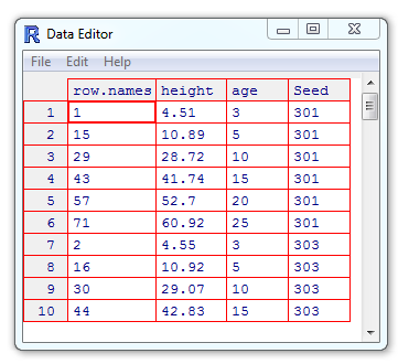
Figure 3.1: The default R spreadsheet editor.

3.6 Facilitating Command Line Data Entry

Command line data entry is made easier with with several R functions. The function scan() speeds up data entry because a prompt is given for each data point, and separators are created by the function itself. Data entries can be separated using the space bar or line breaks. The scan() function will be terminated by a additional blank line or an end of file (EOF) signal. These will be Ctrl$+$D in Unix-alike operating systems and Ctrl$+$Z in Windows.

Below I enter the numbers 1, 2, and 3 as datapoints, separated by spaces, and end data entry using an additional line break. The data are saved as the object a.

a <- scan()
1: 1 2 3
4:
Read 3 items

Sequences can be generated quickly in R using the : operator

1:10

 [1]  1  2  3  4  5  6  7  8  9 10

or the function seq(), which allows additional options

seq(1, 10)

 [1]  1  2  3  4  5  6  7  8  9 10

seq(1, 10, by = 2) # 1 to 10 by two

[1] 1 3 5 7 9

seq(1, 10, length = 4) # 1 to 10 in four evenly spaced points

[1]  1  4  7 10

Entries can be repeated with the function rep(). For example, to repeat the sequence 1 through 5, five times, I could type

rep(c(1:5), 5)

 [1] 1 2 3 4 5 1 2 3 4 5 1 2 3 4 5 1 2 3 4 5 1 2 3 4 5

Note that the first argument in rep(), defines the thing we want to repeat and the second argument, 5, specifies the number of repetitions. I can use the argument each to repeat individual elements a particular number of times.

rep(c(1:5), each = 2)

 [1] 1 1 2 2 3 3 4 4 5 5

We can use seq() and rep() simultaneously to create complex sequences. For instance, to repeat the sequence 1,3,5,7,9,11,13,15,17,19, three times, we could type

rep(seq(1, 20, by = 2), 3)

 [1]  1  3  5  7  9 11 13 15 17 19  1  3  5  7  9 11 13 15 17 19  1  3  5
[24]  7  9 11 13 15 17 19

3.7 Importing Data Into R

While it is possible to enter data into R at the command line, this will normally be inadvisable except for small datasets. In general it will be much easier to import data. R can read data from many different kinds of formats including .txt, and .csv (comma separator) files, and files with space, tab, and carriage return datum separators. I generally organize my datasets using Excel$^{\circledR}$ or some other spreadsheet program (although R can handle much larger datasets than these platforms), then save them as .csv files. I then import the .csv files into R using the read.table(), read.csv(), or scan() functions. The function load() can be used to import data files in .rda data formats, or other R objects. Datasets read into R will generally be of class dataframe and data storage mode list.

The read.table() function can import data organized under a wide range of formats. It’s first three arguments are very important.

file defines the name of the file and directory hierarchy which the data are to be read from.
header is a a logical (TRUE or FALSE) value indicating whether file contains column names as its first line.
sep refers to the type of data separator used for columns. Comma separated files use commas to separate data entries. Thus, in this case sep = ",". Tab separators are specified as "\t". Space separators are specified as spaces, specified as simply " ".

Other useful read.table() arguments include row.names, header, and na.strings. The specification row.names = 1 indicates that the first column in the imported dataset contains row names. The specification header = TRUE, the default setting, indicates that the first row of data contains column names. The argument na.strings = "." indicates that missing values in the imported dataset are designated with periods. By default na.strings = NA.

As an example of read.table() usage, assume that I want to import a .csv file called veg.csv located in folder called veg_data, in my working directory. The first row of veg.csv contains column names, while the first column contains row names. Missing data in the file are indicated with periods. I would type:

read.table("veg_data/veg.csv", sep = ",", header = TRUE, row.names
= 1, na.strings = ".")

As before, note that, as a legacy of its development under Unix, R locates files in directories using forward slashes (or doubled backslashes) rather than single Windows backslashes.

The read.csv function assumes data are in a .csv format. Because the argument sep is unnecessary, this results in a simpler code statement.

read.csv("veg_data\\veg.csv", header = TRUE, row.names
= 1, na.strings = ".")

The function scan() can read in data from an essentially unlimited number of formats, and is extremely flexible with respect to character fields and storage modes of numeric data In addition to arguments used by read.table(), scan() has the arguments

what which describes the storage mode of data e.g., "logical", "integer", etc., or if what is a list, components of variables including column names (see below), and
dec which describes the decimal point character (European scientists and journals often use commas).

Assume that has a column of species names, called species, that will serve as the dataframe’s row names, and 3 columns of numeric data, named site1, site2, and site3. We would read the data in with scan using:

scan("veg.csv", what = list(species = "", site1 = 0, site2 = 0, site3 = 0),
na.strings = ".")

The empty string species = "" in the list comprising the argument what, indicates that species contains character data. Stating that the remaining variables equal 0, or any other number, indicates that they contain numeric data.

The easiest way to import data, if the directory structure is unknown or complex, is to use read.csv() or read.table(), with the file.choose() function as the file argument. For instance, by typing:

df <- read.csv(file.choose())

We can now browse for a .csv files to open that will, following import, be a dataframe with the name df. Other arguments (e.g., header, row.names) will need to be used, when appropriate, to import the file correctly.

3.7.1 Import Using RStudio

RStudio allows direct menu-driven import of file types from a number of spreadsheet and statistical packages including Excel$^{\circledR}$, SPSS$^{\circledR}$, SAS$^{\circledR}$, and Stata$^{\circledR}$ by going to File$>$Import Dataset. We note, however, that restrictions may exist, which may not be present for read.table() and read.csv(). These are summarized in Table 3.6.

Table 3.6: Data import options in RStudio by data storage file type.
	CSV or Text	Excel$^{\circledR}$	SAS$^{\circledR}$, SPSS$^{\circledR}$, Stata$^{\circledR}$
Import from file system or URL	X	X	X
Change column data types	X	X
Skip or include columns	X	X	X
Rename dataset	X	X
Skip the first n rows	X	X
Use header row for column names	X
Trim spaces in names	X
Change column delimiter	X
Encodingselection	X
Select quote identifiers	X
Select escape identifiers	X
Select comment identifiers	X
Select `NA` identifiers	X	X
Specify model file			X

3.7.2 Final Considerations

It is generally recommended that datasets imported and used by R be smaller than 25% of the physical memory of the computer. For instance, they should use less than 8 GB on a computer with 32 GB of RAM. R can handle extremely large datasets, i.e. $> 10$ GB, and $> 1.2 \times 10^{10}$ rows. In this case, however, specific R packages can be used to aid in efficient data handling. Parallel computing and workstation modifications may allow even greater efficiency. The actual upper physical limit for an R dataframe is $2 \times 10^{31}-1$ elements. Note that this exceeds Excel$^{\circledR}$ by 31 orders of magnitude (Excel 2019 worksheets can handle approximately $1.7 \times 10^{10}$ cell elements). R also allows interfacing with a number relational database storage platforms. These include open source entities that express queries in SQL (Structured Query Language). For more information see and .

Exercises

Create the following data structures:
1. An atomic vector object with the numeric entries 1,2,3,4.
2. A matrix object with two rows and two columns with the numeric entries 1,2,3,4.
3. A dataframe object with two columns; one column containing the numeric entries 1,2,3,4, and one column containing the character entries "a","b","c","d".
4. A list containing the objects created in (b) and (c).
5. Using class(), identify the class and the data storage mode for the objects created in problems a-d. Discuss the characteristics of the identified classes.
Assume that you have developed an R algorithm that saves hourly stream temperature sensor outputs greater than $20^\text{o}$ from each day as separate dataframes and places them into a list container, because some days may have several points exceeding the threshold and some days may have none. Complete the following based on the list hi.temps given below:
1. Combine the dataframes in hi.temps into a single dataframe using do.call().
2. Create a dataframe consisting of 10 sets of repeated measures from the dataframe hi.temps$day2 using do.call().

hi.temps <- list(day1 = data.frame(time = c(), temp = c()),
                 day2 = data.frame(time = c(15,16), temp = c(21.1,22.2)),
                 day3 = data.frame(time = c(14,15,16),
                                   temp = c(21.3,20.2,21.5)))

Given the dataframe boo below, provide solutions to the following questions:
1. Identify heights that are less than or equal to 80 inches.
2. Identify heights that are more than 80 inches.
3. Identify females (i.e. F) greater than or equal to 59 inches but less 63 inches.
4. Subset rows of boo to only contain only data for males (i.e. M) greater than or equal to 75 inches tall.
5. Find the mean weight of males who are 75 or 76 inches tall.
6. Use ifelse() or if() to classify heights equal to 60 inches as "small", and heights greater than or equal to 60 inches as "tall".

boo <- data.frame(height.in = c(70, 76, 72, 73, 81, 66, 69, 75, 80, 81,
                                60, 64, 59, 61, 66, 63, 59, 58, 67, 59),
                  weight.lbs = c(160, 185, 180, 186, 200, 156, 163, 178,
                                 186, 189, 140, 156, 136, 141, 158, 154,
                                 135, 120, 145, 117),
                  sex = c(rep("M", 10), rep("F", 10)))

Create x <- NA, y <- NaN, and z <- NULL.
1. Test for the class of x using x == NA and is.na(x) and discuss the results.
2. Test for the class of y using y == NaN and is.nan(y) and discuss the results.
3. Test for the class of z using z == NULL and is.null(z) and discuss the results.
4. Discuss NA, NaN, and NULL designations what are these classes used for and what do they represent?
For the following questions, use data from Table 3.7 below.
1. Write the data into an R dataframe called plant. Use the functions seq() and rep() to help.
2. Use names() to find the names of the variables.
3. Access the first row of data using square brackets.
4. Access the third column of data using square brackets.
5. Access rows three through five using square brackets.
6. Access all rows except rows three, five and seven using square brackets.
7. Access the fourth element from the third column using square brackets.
8. Apply na.omit() to the dataframe and discuss the consequences.
9. Create a copy of plant called plant2. Using square brackets, replace the 7th item in the 2nd column in plant2, an NA value, with the value 12.1.
10. Switch the locations of columns two and three in plant2 using square brackets.
11. Export the plant2 dataframe to your working directory.
12. Convert the plant2 dataframe into a matrix using the function as.matrix. Discuss the consequences.

Table 3.7: Data for Question 5.
Plant height (dm)	Soil N (%)	Water index (1-10)	Management type
22.3	12	1	A
21	12.5	2	A
24.7	14.3	3	B
25	14.2	4	B
26.3	15	5	C
22	14	6	C
31	NA	7	D
32	15	8	D
34	13.3	9	E
42	15.2	10	E
28.9	13.6	1	A
33.3	14.7	2	A
35.2	14.3	3	B
36.7	16.1	4	B
34.4	15.8	5	C
33.2	15.3	6	C
35	14	7	D
41	14.1	8	D
43	16.3	9	E
44	16.5	10	E

Let: \[\boldsymbol{A} = \begin{bmatrix} 2 & -3\\ 1 & 0 \end{bmatrix} \text{and } \boldsymbol{b} = \begin{bmatrix} 1\\ 5 \end{bmatrix} \] Perform the following operations using R:
1. $\boldsymbol{A}\boldsymbol{b}$
2. $\boldsymbol{b}\boldsymbol{A}$
3. $det(\boldsymbol{A})$
4. $\boldsymbol{A}^{-1}$
5. $\boldsymbol{A}'$
We can solve systems of linear equations using matrix algebra under the framework $\boldsymbol{A}\boldsymbol{x} = \boldsymbol{b}$, and (thus) $\boldsymbol{A}^{-1}\boldsymbol{b} = \boldsymbol{x}$. In this notation $\boldsymbol{A}$ contains the coefficients from a series of linear equations (by row), $\boldsymbol{b}$ is a vector of solutions given in the individuals equations, and $\boldsymbol{x}$ is a vector of solutions sought in the system of models. Thus, for the linear equations:

\[\begin{aligned} x + y &= 2\\ -x + 3y &= 4 \end{aligned}\]

we have:

\[\boldsymbol{A} = \begin{bmatrix} 1 & 1\\ -1 & 3 \end{bmatrix}, \boldsymbol{ x} = \begin{bmatrix} x\\ y \end{bmatrix}, \text{ and } \boldsymbol{b} = \begin{bmatrix} 2\\ 4 \end{bmatrix}.\]

Thus, we have \[\boldsymbol{A}^{-1}\boldsymbol{b} = \boldsymbol{x} = \begin{bmatrix} 1/2\\ 3/2 \end{bmatrix}.\]

Given this framework, solve the system of equations below with linear algebra using R.

\[ \begin{aligned} 3x + 2y - z &= 1\\ 2x - 2y + 4z &= -2\\ -x + 0.5y -z &= 0 \end{aligned} \]

Complete the following exercises concerning the R contributed package asbio:
1. Install⁹ and load the package asbio for the current work session.
2. Access the help file for bplot() (a function in asbio).
3. Load the dataset fly.sex from asbio.
4. Obtain documentation for the dataset fly.sex and describe the dataset variables.
5. Access the column longevity in fly.sex using the function with().
Create .csv and .txt datasets, place them in your working directory, and read them into R.

References

Aho, Ken. 2023. Asbio: A Collection of Statistical Tools for Biologists. https://CRAN.R-project.org/package=asbio.

Bates, Douglas, Martin Mächler, Ben Bolker, and Steve Walker. 2015. “Fitting Linear Mixed-Effects Models Using lme4.” Journal of Statistical Software 67 (1): 1–48. https://doi.org/10.18637/jss.v067.i01.

Bates, Douglas, Martin Maechler, and Mikael Jagan. 2023. Matrix: Sparse and Dense Matrix Classes and Methods. https://CRAN.R-project.org/package=Matrix.

Bivand, Roger S., Edzer Pebesma, and Virgilio Gómez-Rubio. 2013. Applied Spatial Data Analysis with R, Second Edition. Springer, NY. https://asdar-book.org/.

Canty, Angelo, and B. D. Ripley. 2022. Boot: Bootstrap r (s-Plus) Functions.

Fox, John, and Sanford Weisberg. 2019. An R Companion to Applied Regression. Third. Thousand Oaks CA: Sage. https://socialsciences.mcmaster.ca/jfox/Books/Companion/.

Hothorn, Torsten, Kurt Hornik, Mark A. van de Wiel, and Achim Zeileis. 2006. “A Lego System for Conditional Inference.” The American Statistician 60 (3): 257–63. https://doi.org/10.1198/000313006X118430.

———. 2008. “Implementing a Class of Permutation Tests: The coin Package.” Journal of Statistical Software 28 (8): 1–23. https://doi.org/10.18637/jss.v028.i08.

Lemon, J. 2006. “Plotrix: A Package in the Red Light District of r.” R-News 6 (4): 8–12.

Maechler, Martin, Peter Rousseeuw, Anja Struyf, Mia Hubert, and Kurt Hornik. 2022. Cluster: Cluster Analysis Basics and Extensions. https://CRAN.R-project.org/package=cluster.

Oksanen, Jari, Gavin L. Simpson, F. Guillaume Blanchet, Roeland Kindt, Pierre Legendre, Peter R. Minchin, R. B. O’Hara, et al. 2022. Vegan: Community Ecology Package. https://CRAN.R-project.org/package=vegan.

Pebesma, Edzer, and Roger S. Bivand. 2023. Spatial Data Science with Applications in R. Chapman & Hall. https://r-spatial.org/book/.

Pinheiro, José C., and Douglas M. Bates. 2000. Mixed-Effects Models in S and S-PLUS. New York: Springer. https://doi.org/10.1007/b98882.

R Core Team. 2023. R: A Language and Environment for Statistical Computing. Vienna, Austria: R Foundation for Statistical Computing. https://www.R-project.org/.

Sarkar, Deepayan. 2008. Lattice: Multivariate Data Visualization with R. New York: Springer. http://lmdvr.r-forge.r-project.org.

Tierney, Luke. 2023. Codetools: Code Analysis Tools for r. https://CRAN.R-project.org/package=codetools.

Venables, W. N., and B. D. Ripley. 2002. Modern Applied Statistics with S. Fourth. New York: Springer. https://www.stats.ox.ac.uk/pub/MASS4/.

Wand, Matt. 2023. KernSmooth: Functions for Kernel Smoothing Supporting Wand and Jones (1995). https://CRAN.R-project.org/package=KernSmooth.

Wickham, Hadley. 2016. Ggplot2: Elegant Graphics for Data Analysis. Springer-Verlag New York. https://ggplot2.tidyverse.org.

———. 2019. Advanced R. CRC press.

Wickham, Hadley, Mara Averick, Jennifer Bryan, Winston Chang, Lucy D’Agostino McGowan, Romain François, Garrett Grolemund, et al. 2019. “Welcome to the tidyverse.” Journal of Open Source Software 4 (43): 1686. https://doi.org/10.21105/joss.01686.

Wikipedia. 2023. “Null Object.” https://en.wikipedia.org/wiki/Null_object_pattern#cite_note-2.

Wood, S. N. 2017. Generalized Additive Models: An Introduction with R. 2nd ed. Chapman; Hall/CRC.

Wood, S. N. 2011. “Fast Stable Restricted Maximum Likelihood and Marginal Likelihood Estimation of Semiparametric Generalized Linear Models.” Journal of the Royal Statistical Society (B) 73 (1): 3–36.

Note that distinctions of these objects are not always clear or consistent (see examples here). For instance, a names attribute can be given to elements of vectors and lists, and columns of dataframes. However, only names from dataframes and lists can be made visible using attach, or called using $.↩︎
Matrices and arrays which, optimally, will both be numeric storage structures, cannot have a names attribute. Instead, row names and column names can be applied using the functions row.names() and col.names(). These, however, cannot be called with attach() or $.↩︎
All objects from a specific class can also be removed from a workspace. For instance, to remove all dataframes one could use: rm(list=ls(all=TRUE)[sapply(mget(ls(all=TRUE)), class) == "data.frame"])↩︎
The numeric class is often used as an alias for class double. In fact, as.numeric() is identical to as.double(), and numeric() is identical to double() (Wickham 2019).↩︎
All numeric objects in R are stored with double-precision, and will require two adjacent locations in computer memory (see Ch 12). Numeric objects coerced to be integers (with as.intger()) will be stored with double precision, although one of the storage locations will not be used. As a result, integers are not conventional double precision data.↩︎
Coercion can also be implemented using class generating functions described earlier. For instance, data.frame(matrix(nrow = 2, data = rnorm(4))) converts a $2 \times 2$ matrix into an equivalent dataframe.↩︎
For instance, subset() and dplyr::filter().↩︎
This actually isn’t necessary since datasets in the package dataset default to being read into an R-session automatically. This step will be necessary, however, in order to obtain datasets from packages that are not lazy loaded (Ch 10).↩︎
Installation of packages via knitting of RMarkdown or Sweave R code chunks is not allowed. Instead, one should install packages from the console. Packages can be loaded via knitting once they are installed.↩︎

Operator	Operation	To.find.	We.type.
`t()`	Matrix transpose	\(\boldsymbol{A}^T\)	`t(A)`
`%*%`	Matrix multiply	\(\boldsymbol{A} \cdot \boldsymbol{A}\)	`A%*%A`
`det()`	Determinant	\(Det(\boldsymbol{A})\)	`det(A)`
`solve()`	Matrix inverse	\(\boldsymbol{A}^{-1}\)	`solve(A)`

Operator	Operation	To ask:	We type:
`>`	\(>\)	Is `x` greater than `y`?	`x > y`
`>=`	\(\geq\)	Is `x` greater than or equal to `y`?	`x >= y`
`<`	\(<\)	Is `x` less than `y`?	`x < y`
`<=`	\(\leq\)	Is `x` less than or equal to `y`	`x <= y`
`==`	\(=\)	Is `x` equal to `y`?	`x == y`
`!=`	\(\neq\)	Is `x` not equal to `y`?	`x != y`
`&`	and	Do `x` and `y` equal `z`?	`x & y == z`
`&&`	and (control flow)	Do `x` and `y` equal `z`?	`x && y == z`
\|	or	Do `x` or `y` equal `z`?	`x` \| `y == z`
\|\|	or (control flow)	Do `x` or `y` equal `z`?	`x` \|\| `y == z`