Chapter 2 Some Basics

“Learning to write programs stretches your mind, and helps you think better."

- Bill Gates, 1955-

2.1 First Steps

Upon opening R in Windows, two things will appear in the console of the R Graphical User Interface (R-GUI)¹. These are the license disclaimer (blue text at the top of the console) and the command line prompt, i.e., \(>\) (Fig 2.1). The prompt indicates that R is ready for a command. All commands in R must begin at \(>\).

The appearance of this simple interface will vary slightly among operating systems. In the Windows R-GUI, the command line prompt and user commands are colored red, and output, including errors and warnings, are colored blue. In Mac OS, the command line prompt will be purple, user inputs will be blue, and output will be black. In Unix/Linux, wherein R will generally run from a shell command line, absent of any menus, all three will be black².

We can exit R at any time by typing q() in the console, closing the GUI window (non-Linux only), or by selecting Exit from the pulldown File menu (non-Linux only).

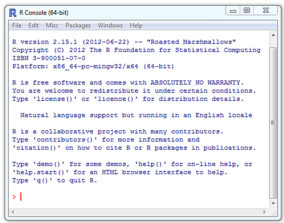
Figure 2.1: An aged, but still recognizable R console: R version 2.15.1, “Roasted Marshmallows”, ca. 2012.

2.2 First Operations

As an introduction we can use R to evaluate a simple mathematical expression. Type 2 + 2 and press Enter.

2 + 2

[1] 4

The output term [1] means, “this is the first requested element.” In this case there is just one requested element, \(4\), the solution to \(2 + 2\). If the output elements cannot be held on a single console line, then R would begin the second line of output with the element number comprising the first element of the new line. For instance, the command rnorm(20) will take 20 random samples from a standard normal distribution (see Ch 3 in Aho (2014)). We have:

rnorm(20)

 [1] -0.83737392 -0.74369931 -0.41155072 -0.16727577 -1.84940106
 [6]  2.19382638  0.17254632 -1.96548697 -0.76901683 -0.03057437
[11]  1.29741329  0.24996308 -0.11678859 -0.04880800  0.21775086
[16] -0.08208237  0.96585536  0.24348213 -1.84999626 -0.01072914

The reappearance of the command line prompt indicates that R is ready for another command. Multiple commands can be entered on a single line, separated by semicolons. Note, however, that this is considered poor programming style, as it may make your code more difficult to understand by a third party.

2 + 2; 3 + 2

[1] 4

[1] 5

R commands are generally insensitive to spaces. This allows the use of spaces to make code more legible. To my eyes, the command 2 + 2 is simply easier to read and debug than 2+2.

2.2.1 Use Your Scroll Keys

As with many other command line environments, the scroll keys (Fig 2.2) provide an important shortcut in R. Instead of editing a line of code by tediously mouse-searching for an earlier command to copy, paste and then modify, you can simply scroll back through your earlier work using the upper scroll key, i.e., \(\uparrow\). Accordingly, scrolling down using \(\downarrow\) will allow you to move forward through earlier commands.

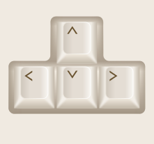
Figure 2.2: Typical scroll direction keys on a keyboard.

2.2.2 Note to Self: #

R will not recognize commands preceded by #. As a result this is a good way for us to leave messages to ourselves.

# Note at beginning of line
2 + 2

[1] 4

2 + # Note in middle of line
+ 2

[1] 4

In the “best” code writing style it is recommended that one place a space after # before beginning a comment, and to insert two spaces following code before placing # in the middle of a line. This convention is followed above.

2.2.3 Unfinished Commands

R will be unable to move on to a new task when a command line is unfinished. For example, type

2 + 

and press Enter. We note that the continuation prompt, +, is now in the place the command prompt should be. R is telling us the command is unfinished. We can get back to the command prompt by finishing the function, clicking Misc\(>\)Stop current computation or Misc\(>\)Stop all computations (non-Linux only) from the R-toolbar, typing Ctrl\(+\)c (Linux only), or by hitting the Esc key (Windows only). Other related shortcuts include Ctrl\(+\)c, which kills a process, and Ctrl\(+\)z, which suspends a process.

2.3 Expressions and Assignments

All entries in R are either expressions or assignments. If a command is an expression it will be evaluated, printed, and discarded. Examples include: 2 + 2. Conversely, an assignment evaluates an expression, and assigns a label to the output, but does not automatically print the result.

To convert an expression to an assignment we use the assignment operator, <-, which represents an arrow that points to the label of the expression. The assignment operator can go on either side of an expression. For instance, if I type:

x <- 2 + 2

or

2 + 2 -> x

then an R-object is created named x that contains the result of the expression 2 + 2. In fact, the code: x <- 2 + 2 literally means: “x is \(2 + 2\).” To print the result (to see x), I simply type:

x

[1] 4

or

print(x)

[1] 4

Note that we could have also typed x = 2 + 2 with the same assignment results.

x = 2 + 2
x

[1] 4

However, for this document, I will continue to use the arrow operator, <-, for object assignments, and save the equals sign, =, for specifying arguments in functions (Ch 8).

Note that the R-console can quickly become cluttered and confusing. To remove clutter on the console (without actually getting rid of any of the objects created in a session) press Ctrl\(+\)L or, from the Edit pulldown menu, click on Clear console (non-Linux only).

2.3.1 Naming Objects

When assigning names to R-objects we should try to keep the names simple, and avoid names that already represent important definitions and functions. These include: TRUE, FALSE, NULL, NA, NaN, and Inf. In addition, we cannot have names:

• beginning with a numeric value,
• containing spaces, colons, and semicolons,
• containing mathematical operators (e.g., *, +, -, ^, /, =),
• containing important R metacharacters (e.g., @, #, ?, !, %, &, |).

Names should, if possible, be descriptive. Thus, for a object containing 20 random observations from a normal distribution, the name rN20 may be superior to the easily-typed, but anonymous name, x. Finally, with assignment commands we should also remember that, like most software developed under Unix/Linux, R is case sensitive. That is, each of the following \(2^4\) combinations will be recognized as distinct: name, Name, nAme, naMe, namE, NAme, nAMe, naME, NaMe, nAmE, NamE, naME, NAMe, nAME, NaME, NAmE, NAME.

2.3.2 Combining Data

To define a collection of numbers (or other data or objects) as a single entity one can use the important R function c, which means “combine”. For instance, to define the numbers 23, 34, and 10 collectively as an object named x, I would type:

x <- c(23, 34, 10)

We could then do something like:

x + 7

[1] 30 41 17

2.3.3 Object Classes

We can view everything created or loaded in R as an object³. Under the idiom of object oriented programming (OOP), an object may have attributes that allow it to be evaluated appropriately, and associated methods appropriate for those attributes (e.g., specific functions for plotting, printing, etc.)⁴.

Currently, I only have the object x in my session:

# type:
objects()

[1] "fc" "x" 

#or
ls()

[1] "fc" "x" 

R objects will generally have a class, identifiable with the function class().

class(x)

[1] "numeric"

Objects in class numeric and several other common classes can be evaluated mathematically. Common R classes are shown in Table 2.1. We will create objects from all of these classes, and learn about their characteristics, over the next few chapters.

Table 2.1: Common R classes for some object x. The listed class would be printed if one created the assignment for x shown in the Example, and typed class(x)

Class	Example
logical	x <- TRUE
numeric	x <- 2 + 2
integer	x <- 1:3
character	x <- c("a","b","c")
factor	x <- factor("a","a","b")
complex	x <- 5i
expression	x <- expression(x * 4)
function	x <- function(y)y + 1
matrix	x <- matrix(nrow = 2, rnorm(4))
array	x <- array(rnorm(8), c(2, 2, 2))
data.frame	x <- data.frame(v1 = c(1,2), v2 = c("a","b"))
list	x <- list()

2.3.4 Object Base Types

All R objects will have so-called base types that identify their underlying C language data structures. Base types of numeric objects define their storage mode, i.e., the way R caches them in its primary memory. Base types can be identified using the function typeof().

typeof(x)

[1] "double"

We see that x has storage mode "double", meaning that its numeric values are stored using up to 53 bits, resulting in recognizable and distinguishable values between approximately \(5 \times 10^{-323}\) and \(2 \times 10^{307}\) (see Ch 12 for more information).

There are currently 25 base types used by R, and it is unlikely that more will be developed in the near future. Some of the more widely-used base types are listed in Table 2.2, following the approach used by (Wickham 2019). The meaning of and usage of some of the base types may seem clear, for instance, integer, character, and character, which are also class designations (Table 2.1). Other base types are be addressed in greater detail in later chapters, including list, logical, integer, and NULL (Ch 3), and environment, pairlist, closure, special, and builtin (Ch 8).

Table 2.2: Common R base types for some object x. The listed base type would be printed if one created the assignment for x shown in the Example and typed typeof(x).

Base type	Example	Application	C type equivalency
NULL	x <- NULL	vectors	NILSXP
logical	x <- TRUE	vectors	LGLSXP
integer	x <- 1L	vectors	INTSXP
complex	x <- 1i	vectors	CPLXSXP
double	x <- 1	vectors	REALXSP
list	x <- list()	vectors	VECXSP
character	x <- "a"	vectors	STRXSP
raw	x <- raw(2)	vectors	RAWSXP
closure	x <- function(y)y + 1	regular functions	CLOSXP
special	x <- `[`	special functions	SPECIALSXP
builtin	x <- sum	primitive functions	BUILTINSXP
expression	x <- expression(x * 4)	expressions	EXPRSXP
environment	x <- globalenv()	environments	EXVSXP
symbol	x <- quote(a)	language components	SYMSXP
language	x <- quote(a + 1)	language components	LANGSXP
pairlist	x <- formals(mean)	language components	LISTSXP

2.3.5 Object Attributes

Many R-objects will also have attributes (i.e., characteristics particular to the object or object class). Typing:

attributes(x)

NULL

indicates that x does not have additional attributes. However, using coercion (Ch 3) we can define x as an object of class matrix (a collection of data in a row and column format, see Ch 3).

attributes(as.matrix(x))

$dim
[1] 3 1

Now x has the attribute dim (i.e., dimension). Specifically, x is a three-celled matrix. It has three rows and one column.

Amazingly, classes and attributes allow R to simultaneously store and distinguish objects with the same name. For instance:

mean <- mean(c(1, 2, 3))
mean

[1] 2

mean(c(1, 2, 3))

[1] 2

In general, it is not advisable to name objects after frequently used functions. Nonetheless, the function mean(), which calculates the arithmetic mean of a collection of data, is distinguishable from the new user-created object mean, because these objects have different identifiable class characteristics. We can remove the user-created object mean, with the function rm(). This leaves behind only the function mean().

rm(mean)
mean

function (x, ...) 
UseMethod("mean")
<bytecode: 0x0000020c59ead508>
<environment: namespace:base>

2.4 Getting Help

There is no single perfect source for information/documentation for all aspects of R. Detailed information concerning basic operations and package development are described at the website (http://www.r-project.org/), but this is generally intended for those familiar with Unix/Linux systems and command line based formats. Thus, this information may not be especially helpful to biologists who are new to R.

2.4.1 help() and ?

A comprehensive help system is built into R. The system can be accessed via the question mark (?) and help() functions. For instance, if I wanted to know more about the plot() function, I could type:

?plot

or

help(plot)

Documentation for functions will include a list of arguments for functions, and a description of variables for datasets, and other pertinent information. Quality of documentation will generally be excellent for functions from packages in the default R download (i.e., the R-distribution packages), but will vary from package to package otherwise. A list of arguments for a function, and their default values, can (often) be obtained using the function formals().

formals(plot)

$x


$y


$...

For help and documentation concerning programming metacharacters used in R (for instance @, #, ?, !, %, &, |), one would enclose the metacharacters with quotes. For example, to find out more information about the logical operator & I could type help("\&") or ? "&". Placing two question marks in front of a topic will cause R to search for help files concerning with respect to all packages in a workstation. For instance, type:

??lm

or, alternatively

help.search(lm)

for a huge number of help files on linear model functions identified through fuzzy matching. Help for particular R-questions can often be found online using the search engine at (http://search.r-project.org/). This link is provided in the Help pulldown menu in the R console (non-Linux only). Helpful online discussions can also be found at Stack Overflow, and Stats Exchange.

2.4.2 demo() and example()

The function demo() allows one access to coded examples that developers have worked out for a particular function or topic. For instance, type:

demo(graphics)

for a brief demonstration of R graphics. Typing

demo(persp)

will provide a demonstration of 3D perspective plots. And, typing:

demo(Hershey)

will provide a demonstration of available modifiable symbols from the Hershey family of fonts . Finally, typing:

demo()

lists all of the demos available in the loaded libraries for a particular workstation. The function example() usually provides less involved demonstrations from the man package directories (short for user manual) in an R package. For instance, type:

example(plotmath)

for a coded demonstration of mathematical graphics.

2.4.3 Vignettes

R packages often contain vignettes. These are short documents that generally describe the theory underlying algorithms and guidance on how to correctly use package functions. Vignettes can be accessed with the function vignette(). To view all available vignettes for packages attached for a current work session, type:

vignette(all = FALSE)

To view all vignettes for all installed packages, type:

vignette(all = TRUE)

To view all vignettes for the installed package asbio, type:

vignette(package = "asbio")

To see the vignette simpson in package asbio, type:

vignette("simpson", package = "asbio")

The function browseVignettes() provides an HTML-browser that allows interactive vignette searches.

2.5 Options

To enhance an R session, we can adjust the appearance of the R-console and customize options that affect expression output. These include the characteristics of the graphics devices, the width of print output in the R-console, and the number of print lines and print digits. Changes to some of these parameters can be made by going to Edit\(>\)GUI Preferences in the R-toolbar. Many other parameters can be changed using the options() function. To see all alterable options one can type:

options()

The resulting list is extensive. To modify options, one would simply define the desired change within parentheses following a call to options. For instance, to see the default number of digits, I would type:

options("digits")

$digits
[1] 7

To change the default number of digits in output from 7 to 5 in the current session, I would type:

options(digits = 5)
# demonstration using pi
pi

[1] 3.1416

One can revert back to default options by restarting an R session.

2.5.1 Advanced Options

To define user-defined options and start up procedures, an.Rprofile file will exist in your R program etc directory. In Windows, this location would be something like: \(\ldots\)R/R-version/etc. R will silently run commands in the .Rprofile file upon opening. Thus, by customizing the .Rprofile file, one can set session options, load installed packages, packages, define your favorite package repository, and even create aliases and defaults for frequently used functions. Here is the content of my current .Rprofile file.

options(repos = structure(c("http://ftp.osuosl.org/pub/cran/")))
.First <- function(){
library(asbio)
cat("\nWelcome to R Ken! ", date(), "\n")
}
.Last <- function(){
cat("\nGoodbye Ken", date(), "\n")
}

The options(repos = structure(c("http://ftp.osuosl.org/pub/cran/"))) command defines my favorite R-repository. The function .First( ) will be run at the start of the R session and .Last( ) will be run at the end of the session. R functions will be addressed in much greater detail in Ch 8. As we go through this primer it will become clear that these functions force R to say hello and to load the package asbio, and print the date/time (using the function date()) when it opens, and to say goodbye, and print the date/time when it closes (although the farewell will only be seen when running R from a command line interface). The .Rprofile file in the /etc directory is the so-called .Rprofile.site file. Additional .Rprofile files can be placed in the working and user directories. R will check for these and run them after running an .Rprofile.site file. One can create .Rprofile files, and many other types of R extension files using the function file.create(). For instance, the code:

file.create("defaults.Rprofile")

places an empty, editable,.Rprofile file called defaults in my working directory.

2.6 The Working Directory

By default, the R working directory is set to be the home directory of the workstation. The command getwd() shows the current file path for the working directory.

getwd()

The working directory can be changed with the command setwd(filepath), where filepath is the location of the desired directory, or by using pulldown menus, i.e., File\(>\)Change dir (non-Linux only). Because R developed under Unix, we must specify directory hierarchies using forward slashes or by doubling backslashes. For instance, to establish a working directory file path to the Windows folder: , I would type:

setwd("C:/Users/User/Documents")

or

setwd("C:\\Users\\User\\Documents")

If one is working in RStudio, the working directory will be set to the location of a R project (Section 2.9).

2.7 Saving and Loading Your Work

As noted in Ch 1, an R session is allocated with a fixed amount of memory that is managed in an on-the-fly manner. An unfortunate consequence of this is that if R crashes, all unsaved information from the work session will be lost. Thus, session work should be saved often. Note that R will not give a warning if you are writing over session files from the R console. The old file will simply be replaced. Three general approaches for saving non-graphics data are possible. These are: 1) saving the history, 2) saving objects, and saving R script. All three of these operations can be greatly facilitated by using an R integrated development environment (IDE) like RStudio (Section 2.9).

2.7.1 R History

To view the history (i.e., the commands that have been used in a session) one can use history(n) where n is the number of previous command lines one wishes to see⁵. For instance, to see the last three commands, one would type:

history(3)

To save the session history in Windows one can use File\(>\)Save History or the function savehistory(). For instance, to save the session history to the working directory under the name history1, I could type:

savehistory(file = "history1.Rhistory")

We can view the code in this file from any text editor. To load the history from a previous session one can use File\(>\)Load History (non-Linux only) or the function loadhistory(). For instance, to load history1 I would type:

loadhistory(file = "history1.Rhistory")

To save the history at the end of (almost) every interactive Windows or Unix-alike R session, one can alter the .Rprofile file .Last function to include:

.Last <- function() if(interactive()) try(savehistory("~/.Rhistory"))

2.7.2 R Objects

To save all of the objects available in the current R-session one can use File\(>\)Save Workspace (non-Linux only), or simply type:

save.image()

This procedure saves session objects to the working directory as a nameless file using an .RData extension. The file will be opened, silently, with the inception of the next R- session, and cause objects used or created in the previous session to be available. Indeed, R will automatically execute all .RData files in the working directory for use in a session. Stored .RData files can also be loaded using File\(>\)Load Workspace (non-Linux only). One can also save .RData objects to a specific directory location and use a specific file name using: File\(>\)Save Workspace, or with flexible function save(). R data file formats, including .rda, and .RData, (extensions for R data files), and .R (the format for R scripts), can be read into R using the function load(). Users new to a command line environment will be reassured by typing:

load(file.choose())

The function file.choose() will allow one to browse interactively for files to load using dialog boxes. Detailed procedures for importing (reading) and exporting (saving) data with a row and column format, and an explicit delimiter (e.g. .csv files) are described in Ch 3.

2.7.3 R Scripts

To save an R script as an executable source file, it is best to use an integrated development environment (IDE) compatible with R. R contains its own IDE, the R-editor, which is useful for writing, editing, and saving scripts as .r extension files. To access the R-editor go to File\(>\)New script (non-Linux only) or type the shortcut Ctrl\(+\)F\(+\)N (Fig 2.3). Code written in the R IDE can be sent directly to the R-console by copying and pasting or by selecting code and using the shortcut Ctrl\(+\)R.

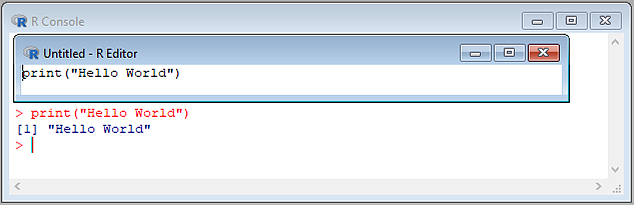
Figure 2.3: The R-editor providing code for a famous computational exercise.

Aside from the R-editor, a number of other IDEs outside of allow straightforward generation of R script files, and a direct link between text editors, that provide syntax highlighting for R code, and the R-console itself. These include RWinEdt (an R package plugin for WinEdt, (http://cran.r-project.org/web/packages/RWinEdt/)), Tinn-R (a recursive acronym for Tinn is not Notepad, (http://www.sciviews.org/Tinn-R)), ESS (Emacs Speaks Statistics, (http://ess.r-project.org)) and particularly RStudio (http://rstudio.org), which will be introduced later in this chapter⁶.

Saved R scripts can be called and executed using the function source(). To browse interactively for source code files, one can type:

source(file.choose())

or go to File\(>\)Source R code.

2.8 Basic Mathematics

A large number of mathematical operators and functions are available with a conventional download of R.

Elementary mathematical operators, common mathematical constants, trigonometric functions, derivative functions, integration approaches, and basic statistical functions are shown in shown in Tables 2.3 - 2.9.

2.8.1 Elementary Operations

Table 2.3: Elementary mathematical operators and functions in R. For all functions x represents a scalar or a numeric vector.

Operator	Operation	To find:	We type:
+	addition	\(2 + 2\)	2 + 2
-	subtraction	\(2 - 2\)	2 - 2
*	multiplication	\(2 \times 2\)	2 * 2
/	division	\(\frac{2}{3}\)	2/3
%%	modulo	remainder of \(\frac{5}{2}\)	5%%2
%/%	integer division	\(\frac{5}{2}\) without remainder	5%/%2
^	exponentiation	\(2^3\)	2^3
abs(x)	\(\mid x \mid\)	\(\mid -23.7 \mid\)	abs(-23.7)
round(x, digits = d)	round \(x\) to \(d\) digits	round \(-23.71\) to 1 digit	round(-23.71, 1)
ceiling(x)	round \(x\) up to closest whole num.	ceiling(2.3)	ceiling(2.3)
floor(x)	round \(x\) down to closest whole num.	floor(2.3)	floor(2.3)
sqrt(x)	\(\sqrt{x}\)	\(\sqrt{2}\)	sqrt(2)
log(x)	\(\log_e{x}\)	\(\log_e{5}\)	log(5)
log(x, base = b)	\(\log_b{x}\)	\(\log_{10}{5}\)	log(5, base = 10)
factorial(x)	\(x!\)	\(5!\)	factorial(5)
gamma(x)	\(\Gamma(x)\)	\(\Gamma(3.2)\)	gamma(3.2)
choose(n,x)	\(\binom{n}{x}\)	\(\binom{5}{2}\)	choose(5,2)
sum(x)	\(\sum_{i=1}^{n}x_i\)	sum of x	sum(x)
cumsum(x)	cumulative sum	cum. sum of x	cumsum(x)
prod(x)	\(\prod_{i=1}^{n}x_i\)	product of x	prod(x)
cumprod(x)	cumulative product	cum. prod. of x	cumprod(x)

2.8.2 Associativity and Precedence

Note that the operation:

2 + 6 * 5

[1] 32

is equivalent to \(2 + (6 \cdot 5) = 32\). This because the * operator gets higher priority (precedence) than +. This can be modified with parentheses:

(2 + 6) * 5

[1] 40

In the absence of operator precedence, mathematical operations R are (generally) read from left to right (that is, their associativity is from left to right) (Table 2.4). This corresponds to the conventional order of operations in mathematics. For instance:

1 + 2^(2 + 1)

[1] 9

Table 2.4: Precedence and associativity of mathematical operators. Operators are listed from highest to lowest precendece in operations.

Precedent	Operator	Description	Associativity
1	^	exponent	right to left
2	%%	modulo	left to right
3	* /	multiplication, division	left to right
4	+ -	addition, subtraction	left to right

2.8.3 Funtion Arguments

R functions generally require a user to specify arguments (in parentheses) following the function name. For instance, sqrt() and factorial() each require one argument, a call to data itself. Thus, to solve \(1/\sqrt{22!}\), I could type:

1/sqrt(factorial(22))

[1] 2.9827e-11

To solve \(\Gamma \left( \sqrt[3]{23\pi} \right)\), I could type:

gamma((23 * pi)^(1/3))

[1] 7.411

By default the function log() computes natural logarithms, i.e.,

log(exp(1))

[1] 1

The log() function can also compute logarithms to a particular base by specifying the base in an optional second argument called base. For instance, to solve the operation: \(\log_{10}3 + \log_{3}5\), one could type:

log(3, 10) + log(5, 3)

[1] 1.9421

Arguments can be specified by the order that they occur in the list of arguments in the function code, or by calling the argument by name. In the code above I know that the first argument in log() is a call to data, and the second argument defines the base. I may not, however, remember the argument order in a function, or may wish to only change certain arguments from a large allotment. In this case it is better to specify an argument by calling its name and defining its value with an equals sign.

log(x = 3, base = 10) + log(x = 5, base = 3)

[1] 1.9421

2.8.4 Custom Operators

Importantly, one can create personalized operators using a `% operator name %` call to a customized R function (note the use of the accent grave character, `). For instance, the custom operator,`% my.op %` below, squares the first number in the operation and adds this result to the square root of the second number in the operation.

`%my.op%` <- function(a,b){a^2 + sqrt(b)} 
0 %my.op% 4 # 0^2 + sqrt(4)

[1] 2

2 %my.op% 3 # 2^2 + sqrt(3)

[1] 5.7321

Functions will be addressed in much greater detail in Ch 8.

2.8.5 Constants

R allows easy access to most conventional constants (Table 2.5).

Table 2.5: Conventional constants in R.

Operator	Operation	To find:	We type:
-Inf	\(-\infty\)	\(-\infty\)	-Inf
Inf	\(\infty\)	\(\infty\)	Inf
pi	\(\pi = 3.141593 \dots\)	\(\pi\)	pi
exp(1)	\(e = 2.718282 \dots\)	\(e\)	exp(1)
exp(x)	\(e^x\)	\(e^3\)	exp(3)

2.8.6 Trigonometry

R assumes that the inputs for trigonometric functions are in radians. Of course degrees can be obtained from radians using \(Degrees = Radians \times 180/\pi\), or conversely \(Radians = Degrees \times \pi /180\) (Table 2.6).

Table 2.6: Trigonometric functions in R. For all functions x represents a scalar or a numeric vector.

Operator	Operation	To find:	We type:
cos(x)	\(\text{cos}(x)\)	\(\text{cos}(3 \text{ rad.})\)	cos(3)
sin(x)	\(\text{sin}(x)\)	\(\text{sin}(45^{\circ})\)	sin(45 * pi/180)
tan(x)	\(\text{tan}(x)\)	\(\text{tan}(3 \text{ rad.})\)	tan(3)
acos(x)	\(\text{acos}(x)\)	\(\text{acos}(45^{\circ})\)	acos(45 * pi/180)
asin(x)	\(\text{asin}(x)\)	\(\text{asin}(3 \text{ rad.})\)	asin(3)
atan(x)	\(\text{atan}(x)\)	\(\text{atan}(45^{\circ})\)	atan(45 * pi/180)

2.8.7 Derivatives

The function D() finds symbolic and numerical derivatives of simple expressions. It requires two arguments, a mathematical function specified as an expression (i.e., an object of class and base type expression, created using the function expression(), that can be evaluated with the function eval()), and the denominator in the difference quotient. Here is an example of how functions expression and eval() are used:

eval(expression(2 + 2))

[1] 4

Of course we wouldn’t bother to use expression() and eval() in such simple applications. Table 2.7 contains specific examples using D().

Table 2.7: Evaluation of derivatives in R.

To find:	We type:
\(\frac{d}{dx}5x\)	D(expression(5 * x), "x")
\(\frac{d^2}{dx^2} 5x^2\)	D(D(expression(5 * x^2), "x"), "x")
\(\frac{\partial}{\partial x} 5xy + y\)	D(expression(5 * x * y + y), "x")

2.8.8 Integration

The function integrate solves definite integrals. It requires three arguments. The first is an R function defining the integrand. The second and third are the lower and upper bounds of integration. Thus, to solve: \[\int^4_2 3x^2dx\] we could type:

f <- function(x){3 * x^2}
integrate(f, 2, 4)

56 with absolute error < 6.2e-13

R functions are explicitly addressed in Ch 8.

2.8.9 Statistics

R, of course, contains a huge number of statistical functions. These will generally require sample data for summarization. Data can be brought into R from spreadsheet files or other data storage files (we will learn how to do this shortly). As we have learned, data can also be assembled in R. For instance,

x <- c(1, 2, 3)

Statistical estimators can be separated into point estimators, which estimate an underlying parameter that has a single true value (from a Frequentist viewpoint), and intervallic estimators, which estimate the bounds of an interval that is expected, preceding sampling, to contain a parameter at some probability (Aho 2014). Point estimators can be further classified as estimators of location, scale, shape, and order statistics (Table 2.8). Measures of location estimate the typical or central value from a sample. Examples include the arithmetic mean and the sample median. Measures of scale quantify data variability or dispersion. Examples include the sample standard deviation and the sample interquartile range (IQR). Shape estimators describe the shape (i.e., symmetry and peakedness) of a data distribution. Examples include the sample skewness and sample kurtosis. Finally, the \(k\)th order statistic of a sample is equal to its \(k\)th-smallest value. Examples include the data minimum, the data maximum, and other quantiles (including the median). Intervallic estimators include confidence intervals (Table 2.9). A huge number of other statistical estimating, modelling, and hypothesis testing algorithms are also available for the R environment. For guidance, see Venables and Ripley (2002), Aho (2014), and Fox and Weisberg (2019), among others.

Table 2.8: Simple point estimators in R. The term x represents a numeric data vector, and y represents a numeric data vector whose elements are paired with those in x. The cipher asbio:: indicates that the function is located in the package asbio.

Function	Acronym	Description	Estimator type
mean(x)	\(\bar{x}\)	arithmetic mean of \(x\)	location
mean(x, trim = t)		trimmed mean of \(x\) for \(0 \leq t \leq 1\).	location
asbio::G.mean(x)	\(GM\)	geometric mean of \(x\)	location
asbio::H.mean(x)	\(HM\)	harmonic mean of \(x\)	location
median(x)	\(\tilde{x}\)	median of \(x\)	location order statistic
asbio::Mode(x)	\(mode(x)\)	mode of \(x\)	location
sd(x)	\(s\)	standard deviation of \(x\)	scale
var(x)	\(s^2\)	variance of \(x\)	scale
cov(x, y)	\(cov(x,y)\)	covariance of \(x\) and \(y\)	scale
cor(x, y)	\(r_{x,y}\)	pearson correlation of \(x\) and \(y\)	scale
IQR(x)	\(IQR\)	interquartile range of \(x\)	scale order statistic
mad(x)	\(MAD\)	median absolute deviation of \(x\)	scale
asbio::skew(x)	\(g_1\)	skew of \(x\)	shape
asbio::kurt(x)	\(g_2\)	kurtosis of \(x\)	shape
min(x)	\(min(x)\)	min of \(x\)	order statistic
max(x)	\(max(x)\)	max of \(x\)	order statistic
quantile(x, prob = p)	\(\hat{F}^{-1}(p)\)	quantile of \(x\) at lower-tailed probability \(p\)	order statistic

Table 2.9: Some intervallic estimators in R. The term x represents a dataset. The cipher asbio:: indicates that the function is located in the package asbio

Function	Description
asbio::ci.mu.z(x, conf, sigma)	Conf. int. for \(\mu\) at level conf. True SD = sigma.
asbio::ci.mu.t(x, conf)	Conf. int. for \(\mu\) at level conf. \(\sigma\) unknown.
asbio::ci.median(x, conf)	Conf. int. for true median at level conf.

2.9 RStudio

RStudio is an open source integrated development environment (IDE) for R (Fig 2.4). RStudio greatly facilitates writing R code, saving and examining R objects and history, and many other processes. These include, but are not limited to, documenting session workflows, writing R package documentation, calling and receiving code from other languages, and even developing web-based graphical user interfaces. RStudio can currently be downloaded at (https://posit.co/products/open-source/rstudio/). Like R itself, RStudio can be used with Windows, Mac, and Unix/Linux operating systems, RStudio has both freeware and commercial versions⁷. We will use the former here.

Figure 2.4: The RStudio logo.

RStudio is generally implemented using a four pane workspace (Fig 2.5). These are: 1) the code editor, 2) R-console, 3) Environment and histories, 4) Plots and other miscellany.

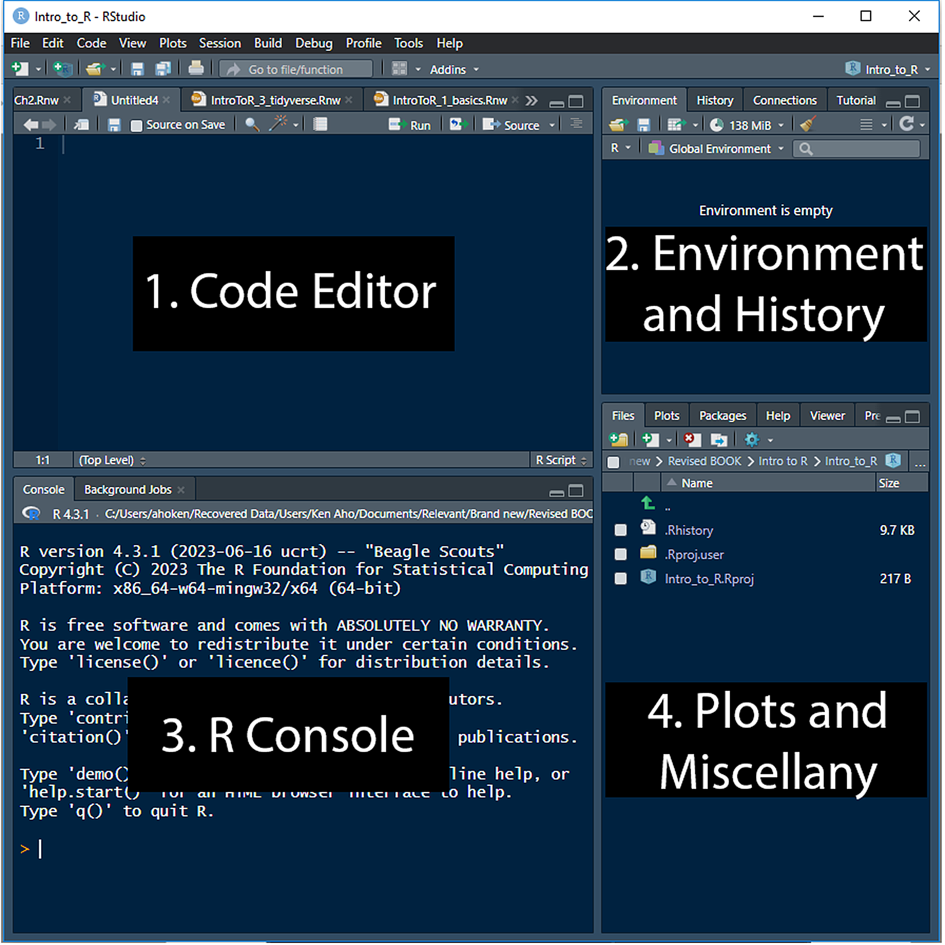
Figure 2.5: Interfaces for RStudio 2023.06.2 Build 561.

• The RStudio code editor panel (Fig 2.5, Panel 1) allows you to create R scripts and scripts for other languages that can be call to and from R. The code panel can also be used to create and edit session documentation files (see below) and other important R file types. A new R script can be created for editing within the code editor withFile\(>\)New\(>\)R Script. Commands from an R script can be sent to the R console using a Ctrl\(+\)Enter shortcut (Windows only).

• The R console panel (Fig 2.5, Panel 2) is identical in functionality to the R console of the most recent version of R on your workstation (assuming that all of the paths and environments are set up correctly on your computer). Thus, the console panel can be used directly for typing and executing R code, or for receiving commands from the code editor (Panel 1).

• The environments and history panel (Fig 2.5, Panel 3) can be used to show: 1) a list of R objects available in your R session, and/or 2) history of all previous commands.

• The plots and files panel (Fig 2.5, Panel 4) can be used to show: 1) files in the working directory (be very careful, as you can permanently delete files from here without (currently) the possibility of recovery from a Recycling Bin), 2) a scrollable history of plots and image files, and 3) a list of available packages. If checked in the GUI list, the package is currently loaded. The panel also has an interface for installing packages. The RStudio File pulldown menu allows straightforward establishment of working directories (although this can still be done at the command line using setwd()). It also provides an interface for point and click import of data files including .csv, .xls, and many other formats (Fig 2.6).

2.9.1 Workflow Documentation

We can document workflow and simultaneously run/test R session code by either:

1. creating an R markdown .rmd file that can be compiled to make a .html, .pdf, or MS Word .doc document⁸, or
2. using Sweave, an approach that implements the LaTeX (pronounced lay-tek) document preparation system.

2.9.1.1 R Markdown

Creating an R Markdown document is simple in RStudio. We first create an empty .rmd document by navigating to File \(>\) New File \(>\)R Markdown (Fig 2.6).

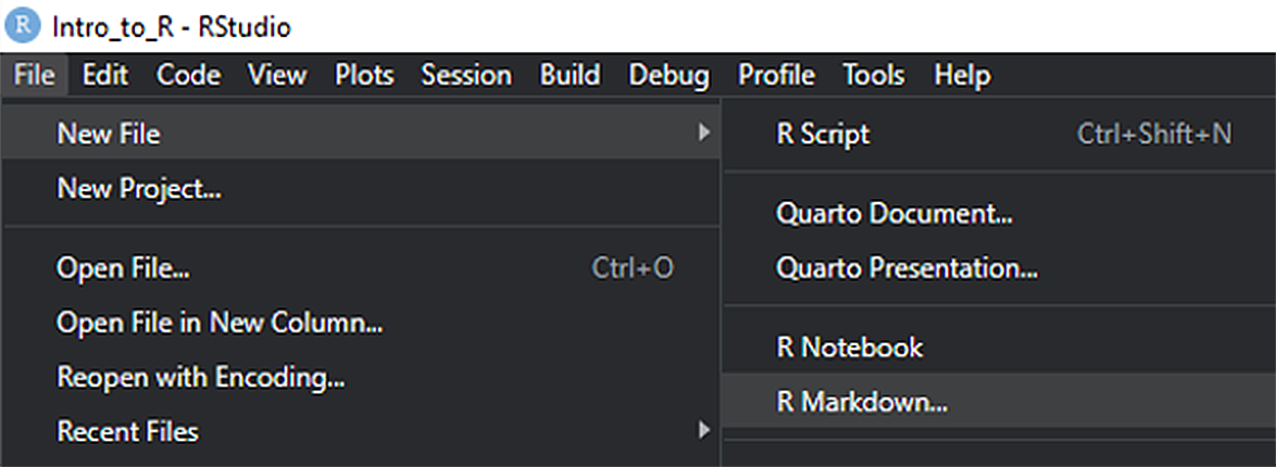
Figure 2.6: Part of the RStudio File pulldown menu.

You will delivered to the GUI shown in Fig 2.7. Note that by default Markdown compilation generates an HTML document.

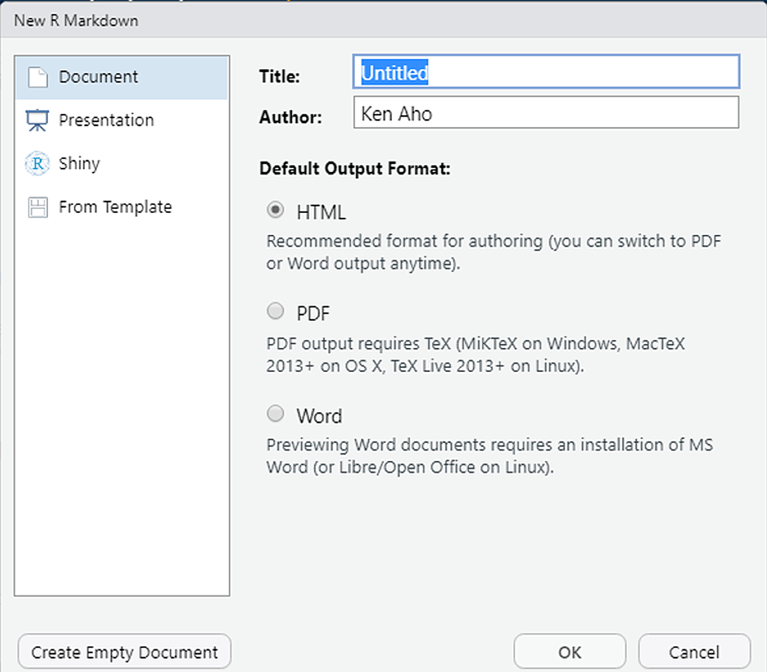
Figure 2.7: RStudio GUI for creating an R Markdown document.

The GUI opens a R Markdown (.rmd) skeleton document. At the top of the .rmd document is a YAML⁹ header that helps to define compiled document characteristics (Fig 2.8). By default an HTML document is created, due to the last line in the header.

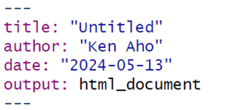
Figure 2.8: YAML header to an R Markdown (.rmd) skeleton document.

This can be changed to one of:

output: pdf_document

or

output: word_document

depending on the style of document one desires.

Markdown lines beginning {```\{r\}} and ending ``` delimit an R code “chunk” to be run in the R environment. The chunk header, {```\{r\}}, can contain additional options. For a complete list of chunk options, run

str(knitr::opts_chunk$get())

Code chunks can be generated by going to Code\(>\)Insert Chunk or by using the RStudio shortcut Ctrl\(+\)Alt\(+\)I. In Markdown, pound signs (e.g., #, ##, ###) can be used as (increasingly nested) hierarchical section delimiters. Additional details on R Markdown can be found at: (http://rmarkdown.rstudio.com).

Inline equations for both Markdown and Sweave (discussed below) can be specified under the LaTeX system, which uses dollar signs, $, to delimit equations. For instance, to obtain the inline equation: \(P(\theta|y) = \frac{P(y|\theta)P(\theta)}{P(y)}\), i.e., Bayes theorem, I could type the LaTeX script:

$(\theta|y) = \frac{P(y|\theta)P(\theta)}{P(y)}$

A cheatsheet for LaTeX equation writing can be found here.

The R Markdown (.rmd) skeleton file has example documentation text, interspersed with example R code in chunks. These been have been modified below to create a simple summary document for the dataset Loblolly from the package datasets (Fig 2.9), which describes growth characteristics of loblolly pine trees (Pinus taeda).

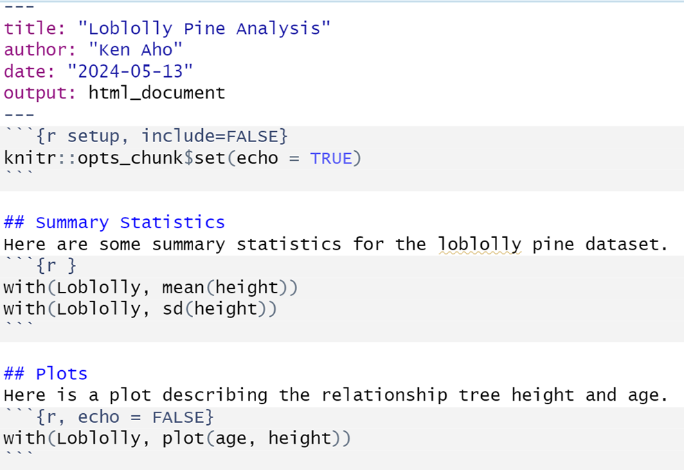
Figure 2.9: An R Markdown (.rmd) file with documentation text and interspersed R code in chunks.

Note the use of echo = FALSE in the second chunk to suppress printing of R code. The knitted HTML is shown in Fig 2.10.

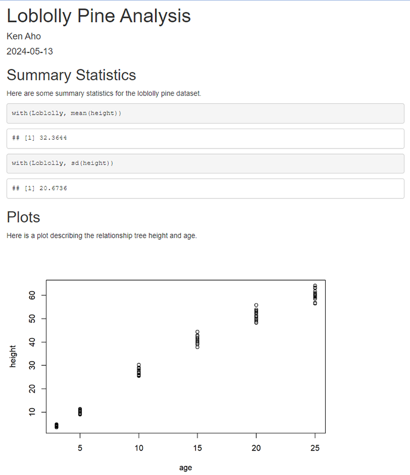
Figure 2.10: An HTML document knit from Markdown code in the previous figure. Note that code is displayed (by default) as well as executed.

A large number of useful auxiliary features are available for Markdown through the R package bookdown (Xie (2016), Xie (2023)). These include the capacity for figure and table numbering and referencing. To use bookdown we must modify the output: designation in the YAML header to be one of the following:

output: bookdown::html_document2

or

output: bookdown::pdf_document2

or

output: bookdown::word_document2

depending on the desired document format.

Among other options, bookdown allows generation of sequentially numbered plots and tables. Numbering R generated plots and tables requires specification of a chunk label after the language reference r. In the chunk below I use the label lobplot. Note that a space is included after r. Captions are specified in the chunk header using the chunk option fig.cap or tab.cap for figures and tables, respectively. For instance,

```{r lobplot, echo=FALSE, fig.cap= "Loblolly pine height versus age."}

Cross-references within the text can be made using the syntax {\@ref(type:label), where label is the chunk label and type is the environment being referenced (e.g., fig, tab, or eq). For the current example, we might want to type something like: “see Figure \@ ref(fig:lobplot)”. in some non-chunk component of the Markdown document. Markdown tables can be created using the function knitr::kable(). For instance,

knitr::kable(head(Loblolly))

	height	age	Seed
1	4.51	3	301
15	10.89	5	301
29	28.72	10	301
43	41.74	15	301
57	52.70	20	301
71	60.92	25	301

As a potential irritation, specification of {output: bookdown::html_document2}, or one of the other two bookdown document options, will result in automated numbering of sections. To turn this numbering off, one could modify the YAML output to be:

output: 
  bookdown::html_document2: 
    number_sections: false

The code indents shown above are important because YAML, like Python, uses significant indentation. To omit numbering for certain sections, one would retain the bookdown output, and add {-} after the unnumbered section heading, e.g.,

# This section is unnumbered {-}

For additional details see: bookdown::html_document2 and the online resource, the R Markdown Cookbook (Xie, Dervieux, and Riederer 2020).

2.9.1.2 Sweave

Under the Sweave documentation approach, high quality .pdf documents are generated from LaTeX .tex files, which in turn are created from Sweave .rnw files. A skeleton .rnw document can be generated by going to File\(>\)New File\(>\)R Sweave¹⁰. In Fig 2.11 I create an .rnw file with the text and analyses used in the Markdown example above (Figs 2.9-2.10). We note that instead of the Markdown YAML header, we now have lines in the preamble defining the type of desired document (e.g., article) and the LaTeX packages needed for document compilation (e.g, amsmath). Note that R code chunks are now enclosed by <<>>=, which serves as a chunk header, and can contain options, and @. Non-code text, including figure and table captions and cross-referencing should follow LaTeX guidelines. Support for LaTeX can be found at the and at a large number of informal user-driven venues, including Stack Exchange and Overleaf, an online LaTeX application.

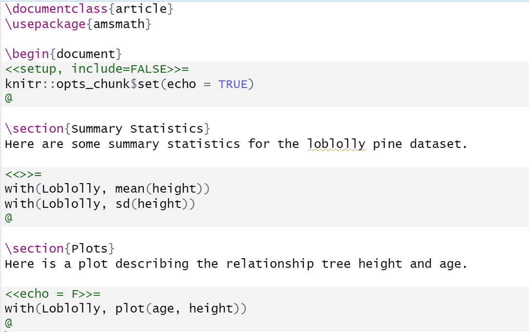
Figure 2.11: A Sweave (.rnw) file with documentation text and interspersed code in chunks.

Fig 2.12 shows the .pdf result, following Sweave/LaTeX compilation.

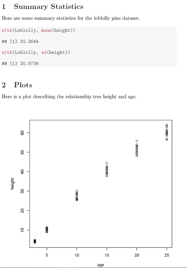
Figure 2.12: A .pdf document resulting from compilation of Sweave code in the previous figure.

2.9.1.3 Purl

R code can be extracted from an .rmd or or an .rnw file using the function knitr::purl.

Exercises

1. Create an R Markdown document to contain your homework assignment. Modify the YAML header to allow numbering of figures and tables, but not sections. To test the formatting, perform the following steps:

   1. Create section header called Question 1 and a subsection header called (a). Under (a) type "completed".
   2. Under the subsection header (b), insert a chunk, and create a simple plot of points at the coordinates: \(\{1,1\}\), \(\{2,2\}\), \(\{3,3\}\), by typing the code: plot(1:3) in the chunk. Create a label for the chunk, and a create caption for plot using the knitr chunk option, fig.cap.
   3. Under the subsection header (c), create a cross reference for the plot from (b).
   4. Under the subsection header (d), write the equation, \(y_i = \hat{\beta}_0 + \hat{\beta}_1x_i + \varepsilon_i\), using LaTeX. As noted earlier, a LaTeX equation cheatsheet can be found here.

Include other assigned exercises for this Chapter as directed, using this general formatting approach given in Question 1.

2. Render (knit) the final document as either an .html file or a .doc file. Perform the following operations.

   1. Leave a note to yourself.
   2. Create and examine an object called x that contains the numeric entries 1, 2, and 3.
   3. Make a copy of x called y.
   4. Show the class of y.
   5. Show the base type of y.
   6. Show the attributes of y.
   7. List the current objects in your work session.
   8. Identify your working directory.

3. Distinguish R expressions and assignments.

4. Sometimes R reports unexpected results for its classes and base types.

   1. Create x <- factor("a","a","b") and show the class of x.
   2. Type ?factor. What is a factor in R?
   3. Show the base type of x? Is this surprising? Why? Type ?integer. What is an integer in R?

5. Solve the following mathematical operations using R.

   1. \(1 + 3/10 + 2\)
   2. \((1 + 3)/10 + 2\)
   3. \(\left(4 \cdot \frac{(3 - 4)}{23}\right)^2\)
   4. \(\log_2(3^{1/2})\)
   5. \(3\boldsymbol{x}^3 + 3\boldsymbol{x}^2 + 2\) where \(\boldsymbol{x} = \{0, 1.5, 4, 6, 8, 10\}\)
   6. \(4(\boldsymbol{x} + \boldsymbol{y})\) where \(\boldsymbol{x} = \{0, 1.5, 4, 6, 8\}\) and \(\boldsymbol{y} = \{-2, 0.5, 3, 5, 8\}\).
   7. \(\frac{d}{dx} \tan(x) 2.3 \cdot e^{3x}\)
   8. \(\frac{d^2}{dx^2} \frac{3}{4x^4}\)
   9. \(\int_3^{12} 24x + \ln(x)dx\)
   10. \(\int_{-\infty}^{\infty} \frac{1}{\sqrt{2\pi}}e^{-\frac{x^2}{2}}dx\) (i.e., find the area under a standard normal pdf).
   11. \(\int_{-\infty}^{\infty}\frac{x}{\sqrt{2\pi}}e^{-\frac{x^2}{2}}dx\) (i.e., find \(E(X)\) for a standard normal pdf).
   12. \(\int_{-\infty}^{\infty}\frac{x^2}{\sqrt{2\pi}}e^{-\frac{x^2}{2}}dx\) (i.e., find \(E(X^2)\) for a standard normal pdf).
   13. Find the sum, cumulative sum, product, cumulative product, arithmetic mean, median and variance of the data x = c(0, 1.5, 4, 6, 8, 10).

6. The velocity of the earth’s rotation on its axis at the equator, \(E\), is approximately \(1700\) km\(\cdot\)hr\(^{-1}\), or 1037 mph. We can calculate the velocity of the rotation of the earth at any latitude with the equation, \(V = \cos(\)latitude\(^\text{o}) \times E\). Using R, simultaneously calculate rotational velocities for latitudes of 0,30,60, and 90 degrees north latitude. Remember, the function cos() assumes inputs are in radians, not degrees.

References

Aho, Ken A. 2014. Foundational and Applied Statistics for Biologists Using R. CRC Press.

Chambers, John M. 2008. Software for Data Analysis: Programming with R. Vol. 2. Springer.

Fox, John, and Sanford Weisberg. 2019. An R Companion to Applied Regression. Third. Thousand Oaks CA: Sage. https://socialsciences.mcmaster.ca/jfox/Books/Companion/.

Venables, W. N., and B. D. Ripley. 2002. Modern Applied Statistics with S. Fourth. New York: Springer. https://www.stats.ox.ac.uk/pub/MASS4/.

Wickham, Hadley. 2019. Advanced R. CRC press.

Xie, Yihui. 2016. Bookdown: Authoring Books and Technical Documents with R Markdown. Boca Raton, Florida: Chapman; Hall/CRC. https://bookdown.org/yihui/bookdown.

———. 2023. Bookdown: Authoring Books and Technical Documents with R Markdown. https://github.com/rstudio/bookdown.

Xie, Yihui, Christophe Dervieux, and Emily Riederer. 2020. R Markdown Cookbook. CRC Press.

---

1. Unix/Linux operating systems require R to be launched from the shell command line by typing: R. This will begin an interactive R session on the system shell command line itself.↩︎

2. A Unix/Linux GUI, similar to those in Windows and Mac OS, can be initiated by opening R with the commands: R -g Tk &.↩︎

3. Although we can view everything created or loaded in R as an object, not all R objects fit neatly into the OOP perspective of “object-oriented.” This is true because R base objects (which are not object oriented) come from S, which was developed before anyone considered the need for an S OOP system (see Wickham (2019) and Chambers (2008)).↩︎

4. There are many OOP languages including R, C#, C++, Objective-C, Smalltalk, Java, Perl, Python and PHP. C is not considered an OOP language.↩︎

5. Importantly, the functions savehistory(), loadhistory(), and history() are not currently supported for Mac OS. There are ways around this. For instance, in RStudio (Section 2.9), the Mac OS command history can be obtained by clicking the History icon that appears on the tool bar at the top of the console window. As an additional issue, Windows and Unix-alike platforms have different implementations for savehistory() and loadhistory(). See help pages for these particular functions within your platform for particulars.↩︎

6. Other text editors with at least some IDE support for R include, but are not limited to, NppToR in Notepad++ (http://sourceforge.net/projects/npptor), Bluefish (http://bluefish.openoffice.nl/index.htm), Crimson Editor (http://www.crimsoneditor.com/), ConTEXT (http://www.contexteditor.org/), Eclipse (http://www.eclipse.org/eclipse/), Vim (http://www.vim.org/), Geany (http://www.geany.org/), jEdit (http://www.jedit.org/), Kate (http://kate-editor.org/), TextMate (http://macromates.com/), gedit (http://projects.gnome.org/gedit/), and SciTE (http://www.scintilla.org/SciTE.html).↩︎

7. On 7/27/2022 RStudio announced it was shifting to a new name, Posit, to acknowledge its growth beyond a simple IDE for R. The RStudio name will be retained for RStudio Desktop, and the RStudio Server, but it will be changed for other applications including the RStudio Workbench (now Posit Workbench) and the RStudio Package Manager (now Posit Package Manager).↩︎

8. Markdown is a highly flexible language for creating formatted text using a plain-text editor. HyperText Markup Language or HTML is the standard markup language for documents designed for web browser display.↩︎

9. YAML is a data serialization language. The YAML acronym was originally intended to mean “Yet Another Markdown Language,” but more recently has been given the recursive acronym: “YAML Ain’t Markup Language.” R Markdown uses a YAML format header to communicate with Pandoc, a document converter embedded in Rstudio. Pandoc can convert markdown syntax, used in an .rmd file, into many formats including .doc and .pdf. This conversion is facilitated by the R package rmarkdown. Specifically, the YAML header passes specific options to rmarkdown::render, to guide the Pandoc document build process.↩︎

10. The document you are reading was either knitted from an RMarkdown .rmd file (using bookdown) or a Sweave .rnw file, created in RStudio.↩︎